How to find the Fourier Transforms of Gaussian and Laplacian filters in OpenCV Python?

We apply Fourier Transform to analyze the frequency characteristics of various filters. We can apply Fourier transform on the Gaussian and Laplacian filters using np.fft.fft2(). We use np.fft.fftshift() to shift the zero-frequency component to the center of the spectrum.

Steps

To find Fourier transforms of the Gaussian or Laplacian filters, you could follow the steps given below ?

• Import the required libraries. In all below Python examples the required Python libraries are OpenCV, NumPy and Matplotlib. Make sure you have already installed them.

• Define a Gaussian or a Laplacian Filter.

• Apply Fourier transform on the above defined filters using np.fft.fft2(filter).

• Call np.fft.fftshift() to shift the zero-frequency component to the center of the spectrum.

• Apply log transform and visualize filters and magnitude spectrum.

Let's look at some examples for a clear understanding about the question.

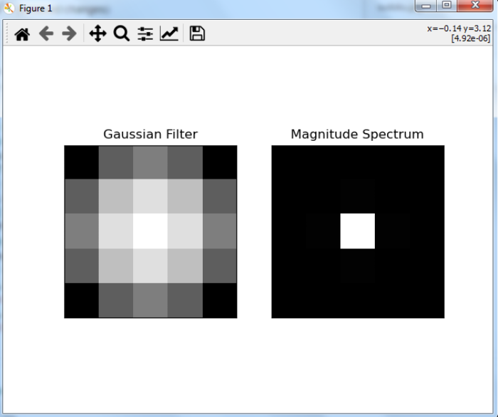
Example 1: Fourier Transform of Gaussian Filter

In this Python program we find the Fourier transform of a Gaussian filter. We also visualize Gaussian filters and Fourier transformed Gaussian filters ?

# import required libraries
import cv2
import numpy as np
from matplotlib import pyplot as plt

# create a Gaussian filter
x = cv2.getGaussianKernel(5, 10)
gaussian = x * x.T

# apply Fourier transform on the Gaussian Filter
fft_filter = np.fft.fft2(gaussian)

# Shift zero-frequency component to the center of the spectrum
fft_shift = np.fft.fftshift(fft_filter)

# apply log transformation
mag_spectrum = np.log(np.abs(fft_shift) + 1)

# visualize the Gaussian filter and transformed Gaussian Filter
plt.subplot(1, 2, 1), plt.imshow(gaussian, cmap='gray')
plt.title('Gaussian Filter'), plt.xticks([]), plt.yticks([])
plt.subplot(1, 2, 2), plt.imshow(mag_spectrum, cmap='gray')
plt.title('Magnitude Spectrum'), plt.xticks([]), plt.yticks([])
plt.show()

The above Python program will produce the following output window ?

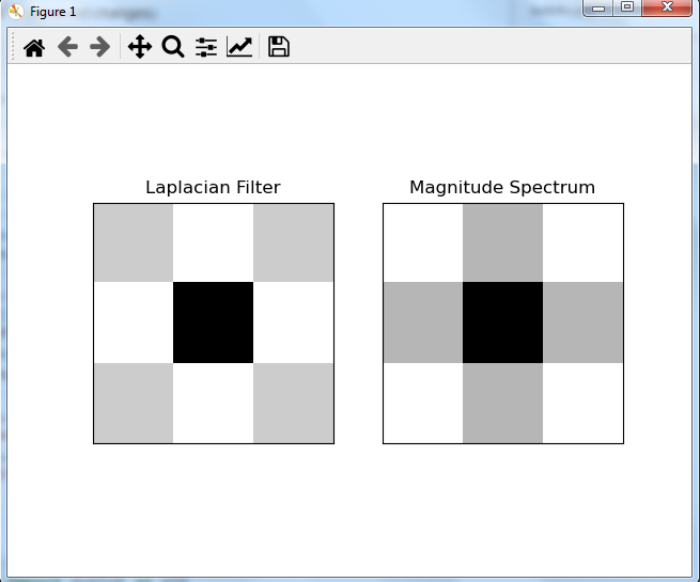
Example 2: Fourier Transform of Laplacian Filter

In this program, we find the Fourier transform of a Laplacian filter. We also visualize Laplacian filters and Fourier transformed Laplacian filters ?

# import required libraries
import cv2
import numpy as np
from matplotlib import pyplot as plt

# create a laplacian Filter
laplacian = np.array([[0, 1, 0], [1, -4, 1], [0, 1, 0]])

# apply Fourier transform on the Laplacian Filter
fft_filter = np.fft.fft2(laplacian)

# shift zero-frequency component to the center of the spectrum
fft_shift = np.fft.fftshift(fft_filter)

# apply log transformation
mag_spectrum = np.log(np.abs(fft_shift) + 1)

# visualize the Laplacian filter and transform Laplacian Filter
plt.subplot(1, 2, 1), plt.imshow(laplacian, cmap='gray')
plt.title('Laplacian Filter'), plt.xticks([]), plt.yticks([])
plt.subplot(1, 2, 2), plt.imshow(mag_spectrum, cmap='gray')
plt.title('Magnitude Spectrum'), plt.xticks([]), plt.yticks([])
plt.show()

It will produce the following output window ?

Key Points

• Gaussian filters are low-pass filters that smooth images by removing high-frequency noise

• Laplacian filters are high-pass filters that enhance edges and detect rapid intensity changes

• The magnitude spectrum shows the frequency distribution of the filter's response

• Log transformation np.log(abs(fft_shift) + 1) helps visualize the wide dynamic range of frequency components

Conclusion

Fourier transforms help analyze filter characteristics in the frequency domain. Use np.fft.fft2() to compute the 2D Fourier transform and np.fft.fftshift() to center the zero-frequency component for better visualization.