Weka - Quick Guide

Weka - Introduction

The foundation of any Machine Learning application is data - not just a little data but a huge data which is termed as Big Data in the current terminology.

To train the machine to analyze big data, you need to have several considerations on the data −

The data must be clean.
It should not contain null values.

Besides, not all the columns in the data table would be useful for the type of analytics that you are trying to achieve. The irrelevant data columns or ‘features’ as termed in Machine Learning terminology, must be removed before the data is fed into a machine learning algorithm.

In short, your big data needs lots of preprocessing before it can be used for Machine Learning. Once the data is ready, you would apply various Machine Learning algorithms such as classification, regression, clustering and so on to solve the problem at your end.

The type of algorithms that you apply is based largely on your domain knowledge. Even within the same type, for example classification, there are several algorithms available. You may like to test the different algorithms under the same class to build an efficient machine learning model. While doing so, you would prefer visualization of the processed data and thus you also require visualization tools.

In the upcoming chapters, you will learn about Weka, a software that accomplishes all the above with ease and lets you work with big data comfortably.

What is Weka?

WEKA - an open source software provides tools for data preprocessing, implementation of several Machine Learning algorithms, and visualization tools so that you can develop machine learning techniques and apply them to real-world data mining problems. What WEKA offers is summarized in the following diagram −

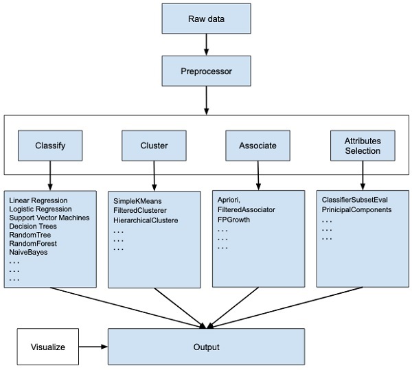
If you observe the beginning of the flow of the image, you will understand that there are many stages in dealing with Big Data to make it suitable for machine learning −

First, you will start with the raw data collected from the field. This data may contain several null values and irrelevant fields. You use the data preprocessing tools provided in WEKA to cleanse the data.

Then, you would save the preprocessed data in your local storage for applying ML algorithms.

Next, depending on the kind of ML model that you are trying to develop you would select one of the options such as Classify, Cluster, or Associate. The Attributes Selection allows the automatic selection of features to create a reduced dataset.

Note that under each category, WEKA provides the implementation of several algorithms. You would select an algorithm of your choice, set the desired parameters and run it on the dataset.

Then, WEKA would give you the statistical output of the model processing. It provides you a visualization tool to inspect the data.

The various models can be applied on the same dataset. You can then compare the outputs of different models and select the best that meets your purpose.

Thus, the use of WEKA results in a quicker development of machine learning models on the whole.

Now that we have seen what WEKA is and what it does, in the next chapter let us learn how to install WEKA on your local computer.

Weka - Installation

To install WEKA on your machine, visit WEKA’s official website and download the installation file. WEKA supports installation on Windows, Mac OS X and Linux. You just need to follow the instructions on this page to install WEKA for your OS.

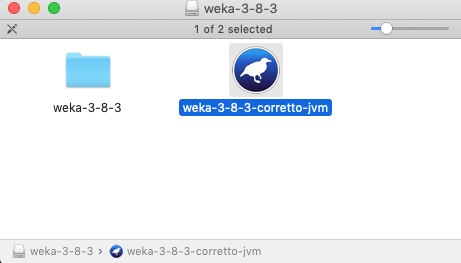
The steps for installing on Mac are as follows −

Download the Mac installation file.
Double click on the downloaded weka-3-8-3-corretto-jvm.dmg file.

You will see the following screen on successful installation.

Click on the weak-3-8-3-corretto-jvm icon to start Weka.
Optionally you may start it from the command line −

java -jar weka.jar

The WEKA GUI Chooser application will start and you would see the following screen −

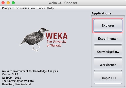
The GUI Chooser application allows you to run five different types of applications as listed here −

Explorer
Experimenter
KnowledgeFlow
Workbench
Simple CLI

We will be using Explorer in this tutorial.

Weka - Launching Explorer

In this chapter, let us look into various functionalities that the explorer provides for working with big data.

When you click on the Explorer button in the Applications selector, it opens the following screen −

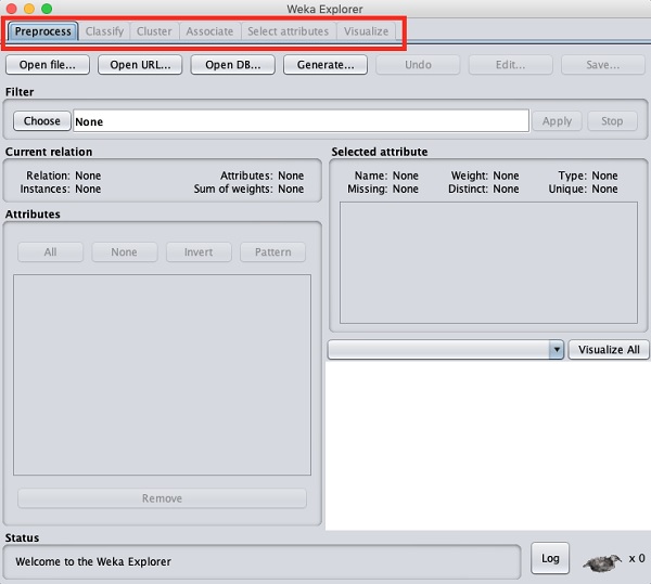
On the top, you will see several tabs as listed here −

Preprocess
Classify
Cluster
Associate
Select Attributes
Visualize

Under these tabs, there are several pre-implemented machine learning algorithms. Let us look into each of them in detail now.

Preprocess Tab

Initially as you open the explorer, only the Preprocess tab is enabled. The first step in machine learning is to preprocess the data. Thus, in the Preprocess option, you will select the data file, process it and make it fit for applying the various machine learning algorithms.

Classify Tab

The Classify tab provides you several machine learning algorithms for the classification of your data. To list a few, you may apply algorithms such as Linear Regression, Logistic Regression, Support Vector Machines, Decision Trees, RandomTree, RandomForest, NaiveBayes, and so on. The list is very exhaustive and provides both supervised and unsupervised machine learning algorithms.

Cluster Tab

Under the Cluster tab, there are several clustering algorithms provided - such as SimpleKMeans, FilteredClusterer, HierarchicalClusterer, and so on.

Associate Tab

Under the Associate tab, you would find Apriori, FilteredAssociator and FPGrowth.

Select Attributes Tab

Select Attributes allows you feature selections based on several algorithms such as ClassifierSubsetEval, PrinicipalComponents, etc.

Visualize Tab

Lastly, the Visualize option allows you to visualize your processed data for analysis.

As you noticed, WEKA provides several ready-to-use algorithms for testing and building your machine learning applications. To use WEKA effectively, you must have a sound knowledge of these algorithms, how they work, which one to choose under what circumstances, what to look for in their processed output, and so on. In short, you must have a solid foundation in machine learning to use WEKA effectively in building your apps.

In the upcoming chapters, you will study each tab in the explorer in depth.

Weka - Loading Data

In this chapter, we start with the first tab that you use to preprocess the data. This is common to all algorithms that you would apply to your data for building the model and is a common step for all subsequent operations in WEKA.

For a machine learning algorithm to give acceptable accuracy, it is important that you must cleanse your data first. This is because the raw data collected from the field may contain null values, irrelevant columns and so on.

In this chapter, you will learn how to preprocess the raw data and create a clean, meaningful dataset for further use.

First, you will learn to load the data file into the WEKA explorer. The data can be loaded from the following sources −

Local file system
Web
Database

In this chapter, we will see all the three options of loading data in detail.

Loading Data from Local File System

Just under the Machine Learning tabs that you studied in the previous lesson, you would find the following three buttons −

Open file …
Open URL …
Open DB …

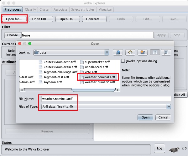
Click on the Open file ... button. A directory navigator window opens as shown in the following screen −

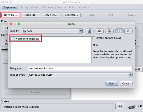
Now, navigate to the folder where your data files are stored. WEKA installation comes up with many sample databases for you to experiment. These are available in the data folder of the WEKA installation.

For learning purpose, select any data file from this folder. The contents of the file would be loaded in the WEKA environment. We will very soon learn how to inspect and process this loaded data. Before that, let us look at how to load the data file from the Web.

Loading Data from Web

Once you click on the Open URL … button, you can see a window as follows −

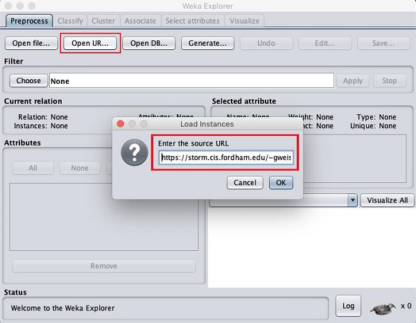
We will open the file from a public URL Type the following URL in the popup box −

https://storm.cis.fordham.edu/~gweiss/data-mining/weka-data/weather.nominal.arff

You may specify any other URL where your data is stored. The Explorer will load the data from the remote site into its environment.

Loading Data from DB

Once you click on the Open DB ... button, you can see a window as follows −

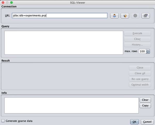
Set the connection string to your database, set up the query for data selection, process the query and load the selected records in WEKA.

Weka - File Formats

WEKA supports a large number of file formats for the data. Here is the complete list −

arff
arff.gz
bsi
csv
dat
data
json
json.gz
libsvm
m
names
xrff
xrff.gz

The types of files that it supports are listed in the drop-down list box at the bottom of the screen. This is shown in the screenshot given below.

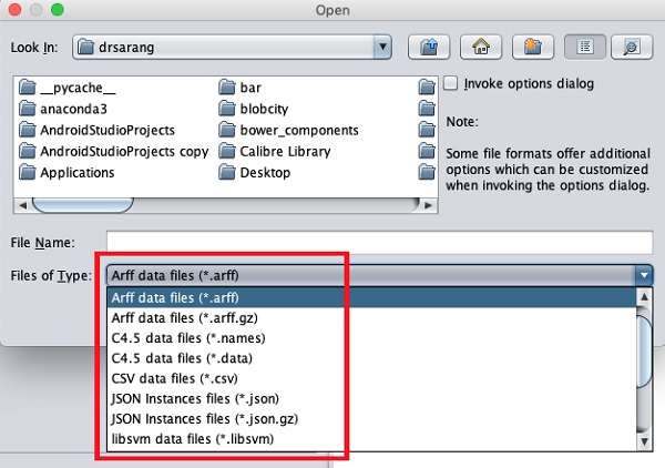
As you would notice it supports several formats including CSV and JSON. The default file type is Arff.

Arff Format

An Arff file contains two sections - header and data.

The header describes the attribute types.
The data section contains a comma separated list of data.

As an example for Arff format, the Weather data file loaded from the WEKA sample databases is shown below −

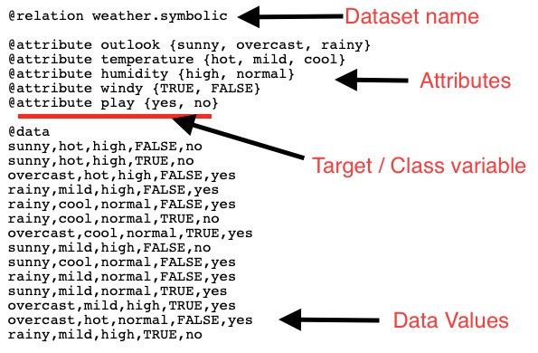
From the screenshot, you can infer the following points −

The @relation tag defines the name of the database.
The @attribute tag defines the attributes.
The @data tag starts the list of data rows each containing the comma separated fields.
The attributes can take nominal values as in the case of outlook shown here −

@attribute outlook (sunny, overcast, rainy)

The attributes can take real values as in this case −

@attribute temperature real

You can also set a Target or a Class variable called play as shown here −

@attribute play (yes, no)

The Target assumes two nominal values yes or no.

Other Formats

The Explorer can load the data in any of the earlier mentioned formats. As arff is the preferred format in WEKA, you may load the data from any format and save it to arff format for later use. After preprocessing the data, just save it to arff format for further analysis.

Now that you have learned how to load data into WEKA, in the next chapter, you will learn how to preprocess the data.

Weka - Preprocessing the Data

The data that is collected from the field contains many unwanted things that leads to wrong analysis. For example, the data may contain null fields, it may contain columns that are irrelevant to the current analysis, and so on. Thus, the data must be preprocessed to meet the requirements of the type of analysis you are seeking. This is the done in the preprocessing module.

To demonstrate the available features in preprocessing, we will use the Weather database that is provided in the installation.

Using the Open file ... option under the Preprocess tag select the weather-nominal.arff file.

When you open the file, your screen looks like as shown here −

This screen tells us several things about the loaded data, which are discussed further in this chapter.

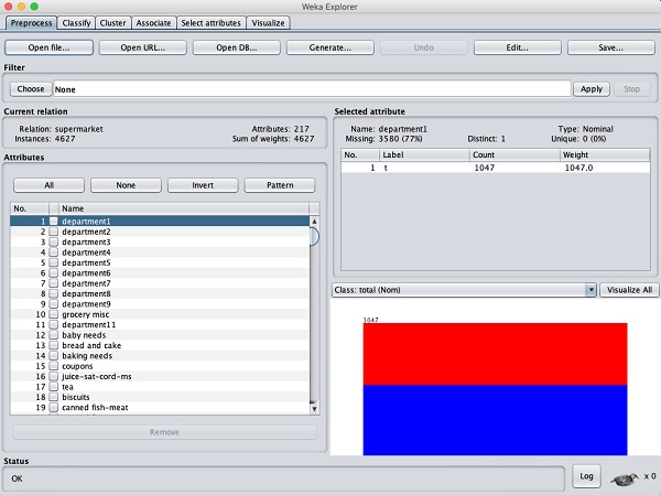
Understanding Data

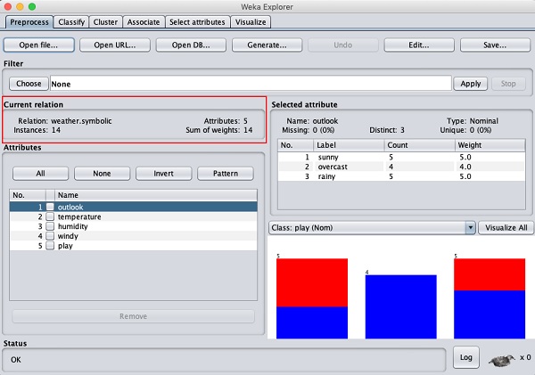
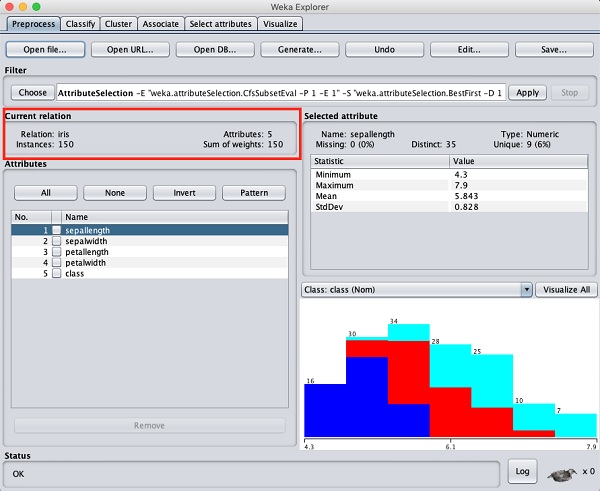
Let us first look at the highlighted Current relation sub window. It shows the name of the database that is currently loaded. You can infer two points from this sub window −

There are 14 instances - the number of rows in the table.
The table contains 5 attributes - the fields, which are discussed in the upcoming sections.

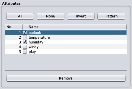
On the left side, notice the Attributes sub window that displays the various fields in the database.

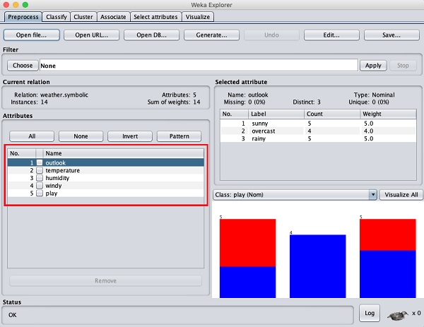
The weather database contains five fields - outlook, temperature, humidity, windy and play. When you select an attribute from this list by clicking on it, further details on the attribute itself are displayed on the right hand side.

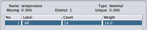
Let us select the temperature attribute first. When you click on it, you would see the following screen −

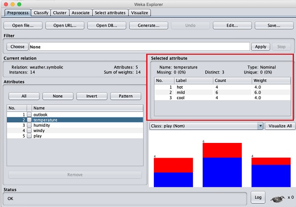
In the Selected Attribute subwindow, you can observe the following −

The name and the type of the attribute are displayed.
The type for the temperature attribute is Nominal.
The number of Missing values is zero.
There are three distinct values with no unique value.
The table underneath this information shows the nominal values for this field as hot, mild and cold.
It also shows the count and weight in terms of a percentage for each nominal value.

At the bottom of the window, you see the visual representation of the class values.

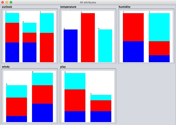
If you click on the Visualize All button, you will be able to see all features in one single window as shown here −

Removing Attributes

Many a time, the data that you want to use for model building comes with many irrelevant fields. For example, the customer database may contain his mobile number which is relevant in analysing his credit rating.

To remove Attribute/s select them and click on the Remove button at the bottom.

The selected attributes would be removed from the database. After you fully preprocess the data, you can save it for model building.

Next, you will learn to preprocess the data by applying filters on this data.

Applying Filters

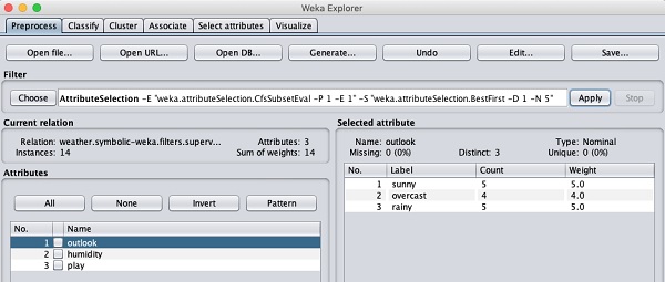
Some of the machine learning techniques such as association rule mining requires categorical data. To illustrate the use of filters, we will use weather-numeric.arff database that contains two numeric attributes - temperature and humidity.

We will convert these to nominal by applying a filter on our raw data. Click on the Choose button in the Filter subwindow and select the following filter −

weka→filters→supervised→attribute→Discretize

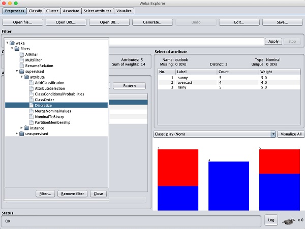
Click on the Apply button and examine the temperature and/or humidity attribute. You will notice that these have changed from numeric to nominal types.

Let us look into another filter now. Suppose you want to select the best attributes for deciding the play. Select and apply the following filter −

weka→filters→supervised→attribute→AttributeSelection

You will notice that it removes the temperature and humidity attributes from the database.

After you are satisfied with the preprocessing of your data, save the data by clicking the Save ... button. You will use this saved file for model building.

In the next chapter, we will explore the model building using several predefined ML algorithms.

Weka - Classifiers

Many machine learning applications are classification related. For example, you may like to classify a tumor as malignant or benign. You may like to decide whether to play an outside game depending on the weather conditions. Generally, this decision is dependent on several features/conditions of the weather. So you may prefer to use a tree classifier to make your decision of whether to play or not.

In this chapter, we will learn how to build such a tree classifier on weather data to decide on the playing conditions.

Setting Test Data

We will use the preprocessed weather data file from the previous lesson. Open the saved file by using the Open file ... option under the Preprocess tab, click on the Classify tab, and you would see the following screen −

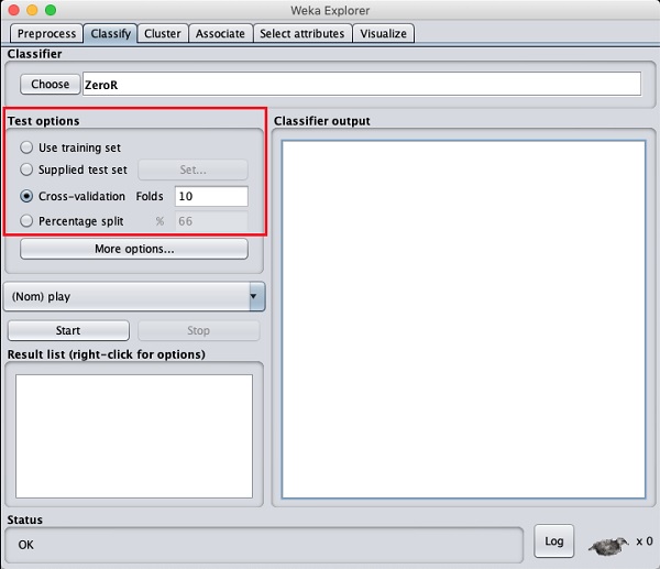
Before you learn about the available classifiers, let us examine the Test options. You will notice four testing options as listed below −

Training set
Supplied test set
Cross-validation
Percentage split

Unless you have your own training set or a client supplied test set, you would use cross-validation or percentage split options. Under cross-validation, you can set the number of folds in which entire data would be split and used during each iteration of training. In the percentage split, you will split the data between training and testing using the set split percentage.

Now, keep the default play option for the output class −

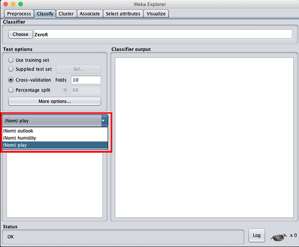
Next, you will select the classifier.

Selecting Classifier

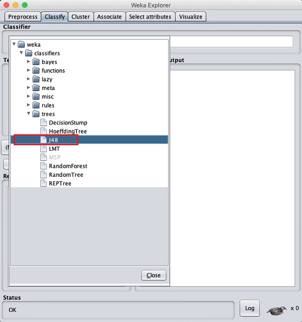
Click on the Choose button and select the following classifier −

weka→classifiers>trees>J48

This is shown in the screenshot below −

Click on the Start button to start the classification process. After a while, the classification results would be presented on your screen as shown here −

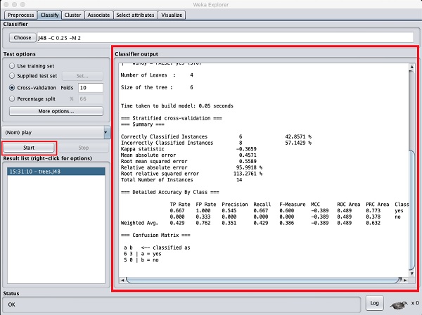
Let us examine the output shown on the right hand side of the screen.

It says the size of the tree is 6. You will very shortly see the visual representation of the tree. In the Summary, it says that the correctly classified instances as 2 and the incorrectly classified instances as 3, It also says that the Relative absolute error is 110%. It also shows the Confusion Matrix. Going into the analysis of these results is beyond the scope of this tutorial. However, you can easily make out from these results that the classification is not acceptable and you will need more data for analysis, to refine your features selection, rebuild the model and so on until you are satisfied with the model’s accuracy. Anyway, that’s what WEKA is all about. It allows you to test your ideas quickly.

Visualize Results

To see the visual representation of the results, right click on the result in the Result list box. Several options would pop up on the screen as shown here −

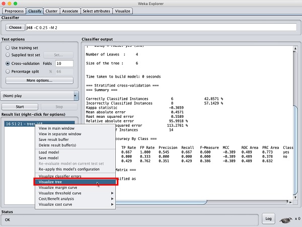
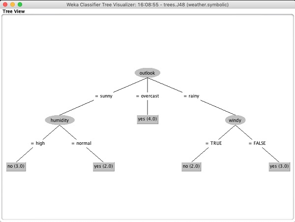
Select Visualize tree to get a visual representation of the traversal tree as seen in the screenshot below −

Selecting Visualize classifier errors would plot the results of classification as shown here −

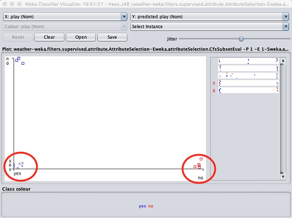
A cross represents a correctly classified instance while squares represents incorrectly classified instances. At the lower left corner of the plot you see a cross that indicates if outlook is sunny then play the game. So this is a correctly classified instance. To locate instances, you can introduce some jitter in it by sliding the jitter slide bar.

The current plot is outlook versus play. These are indicated by the two drop down list boxes at the top of the screen.

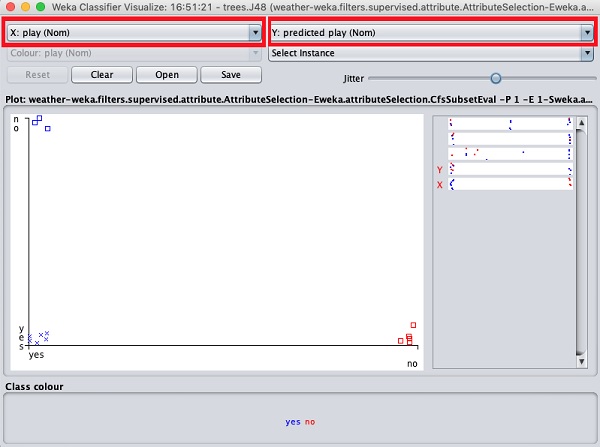
Now, try a different selection in each of these boxes and notice how the X & Y axes change. The same can be achieved by using the horizontal strips on the right hand side of the plot. Each strip represents an attribute. Left click on the strip sets the selected attribute on the X-axis while a right click would set it on the Y-axis.

There are several other plots provided for your deeper analysis. Use them judiciously to fine tune your model. One such plot of Cost/Benefit analysis is shown below for your quick reference.

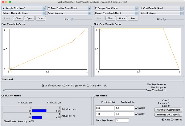
Explaining the analysis in these charts is beyond the scope of this tutorial. The reader is encouraged to brush up their knowledge of analysis of machine learning algorithms.

In the next chapter, we will learn the next set of machine learning algorithms, that is clustering.

Weka - Clustering

A clustering algorithm finds groups of similar instances in the entire dataset. WEKA supports several clustering algorithms such as EM, FilteredClusterer, HierarchicalClusterer, SimpleKMeans and so on. You should understand these algorithms completely to fully exploit the WEKA capabilities.

As in the case of classification, WEKA allows you to visualize the detected clusters graphically. To demonstrate the clustering, we will use the provided iris database. The data set contains three classes of 50 instances each. Each class refers to a type of iris plant.

Loading Data

In the WEKA explorer select the Preprocess tab. Click on the Open file ... option and select the iris.arff file in the file selection dialog. When you load the data, the screen looks like as shown below −

You can observe that there are 150 instances and 5 attributes. The names of attributes are listed as sepallength, sepalwidth, petallength, petalwidth and class. The first four attributes are of numeric type while the class is a nominal type with 3 distinct values. Examine each attribute to understand the features of the database. We will not do any preprocessing on this data and straight-away proceed to model building.

Clustering

Click on the Cluster TAB to apply the clustering algorithms to our loaded data. Click on the Choose button. You will see the following screen −

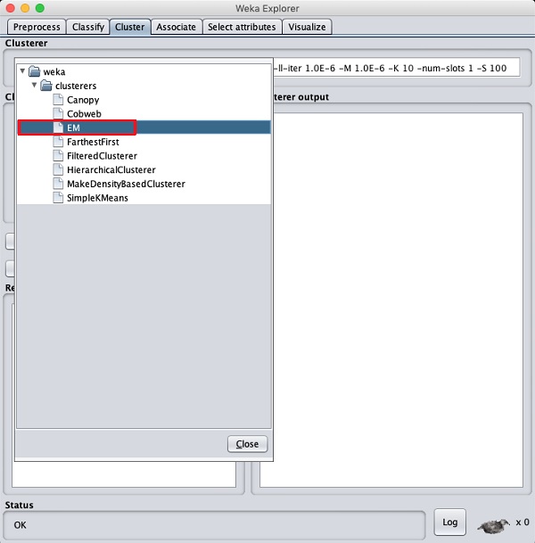
Now, select EM as the clustering algorithm. In the Cluster mode sub window, select the Classes to clusters evaluation option as shown in the screenshot below −

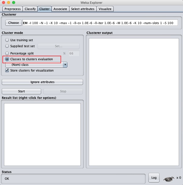
Click on the Start button to process the data. After a while, the results will be presented on the screen.

Next, let us study the results.

Examining Output

The output of the data processing is shown in the screen below −

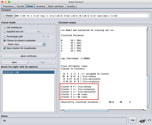
From the output screen, you can observe that −

There are 5 clustered instances detected in the database.
The Cluster 0 represents setosa, Cluster 1 represents virginica, Cluster 2 represents versicolor, while the last two clusters do not have any class associated with them.

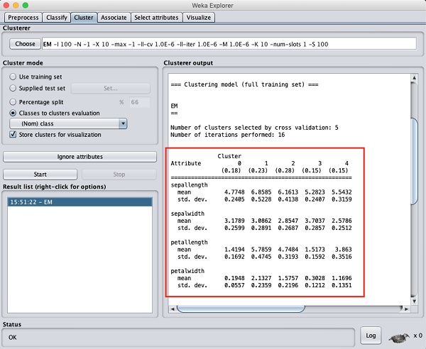
If you scroll up the output window, you will also see some statistics that gives the mean and standard deviation for each of the attributes in the various detected clusters. This is shown in the screenshot given below −

Next, we will look at the visual representation of the clusters.

Visualizing Clusters

To visualize the clusters, right click on the EM result in the Result list. You will see the following options −

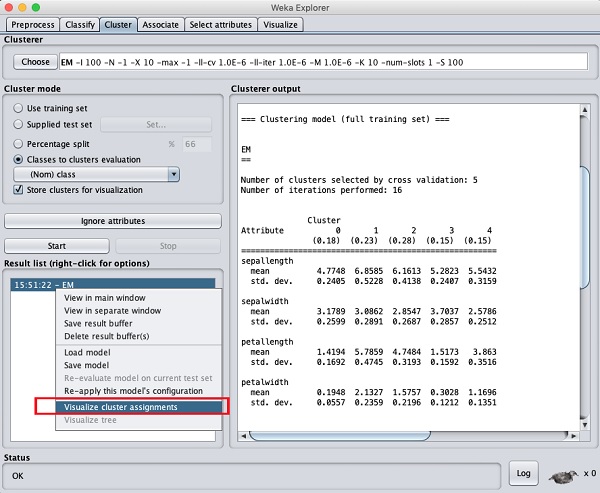
Select Visualize cluster assignments. You will see the following output −

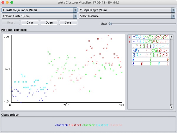
As in the case of classification, you will notice the distinction between the correctly and incorrectly identified instances. You can play around by changing the X and Y axes to analyze the results. You may use jittering as in the case of classification to find out the concentration of correctly identified instances. The operations in visualization plot are similar to the one you studied in the case of classification.

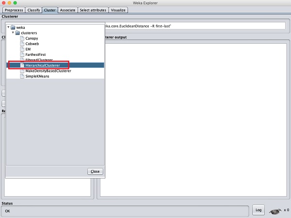
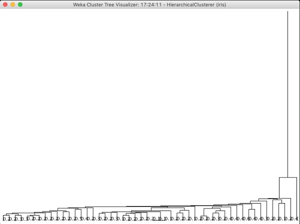
Applying Hierarchical Clusterer

To demonstrate the power of WEKA, let us now look into an application of another clustering algorithm. In the WEKA explorer, select the HierarchicalClusterer as your ML algorithm as shown in the screenshot shown below −

Choose the Cluster mode selection to Classes to cluster evaluation, and click on the Start button. You will see the following output −

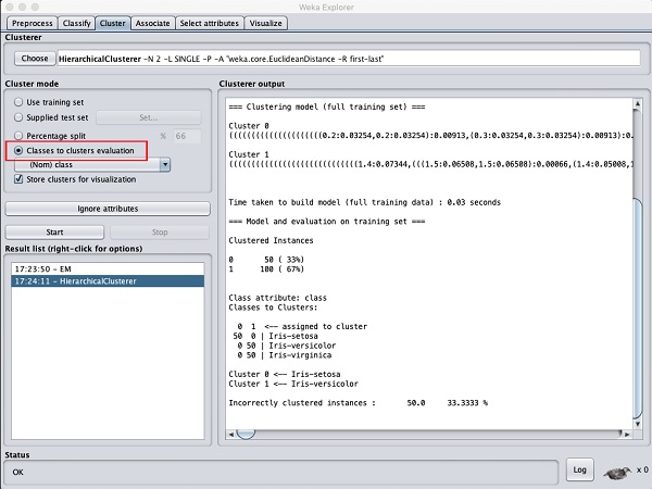
Notice that in the Result list, there are two results listed: the first one is the EM result and the second one is the current Hierarchical. Likewise, you can apply multiple ML algorithms to the same dataset and quickly compare their results.

If you examine the tree produced by this algorithm, you will see the following output −

In the next chapter, you will study the Associate type of ML algorithms.

Weka - Association

It was observed that people who buy beer also buy diapers at the same time. That is there is an association in buying beer and diapers together. Though this seems not well convincing, this association rule was mined from huge databases of supermarkets. Similarly, an association may be found between peanut butter and bread.

Finding such associations becomes vital for supermarkets as they would stock diapers next to beers so that customers can locate both items easily resulting in an increased sale for the supermarket.

The Apriori algorithm is one such algorithm in ML that finds out the probable associations and creates association rules. WEKA provides the implementation of the Apriori algorithm. You can define the minimum support and an acceptable confidence level while computing these rules. You will apply the Apriori algorithm to the supermarket data provided in the WEKA installation.

Loading Data

In the WEKA explorer, open the Preprocess tab, click on the Open file ... button and select supermarket.arff database from the installation folder. After the data is loaded you will see the following screen −

The database contains 4627 instances and 217 attributes. You can easily understand how difficult it would be to detect the association between such a large number of attributes. Fortunately, this task is automated with the help of Apriori algorithm.

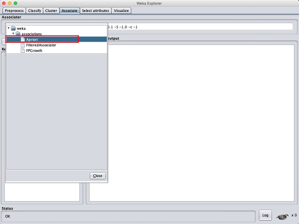
Associator

Click on the Associate TAB and click on the Choose button. Select the Apriori association as shown in the screenshot −

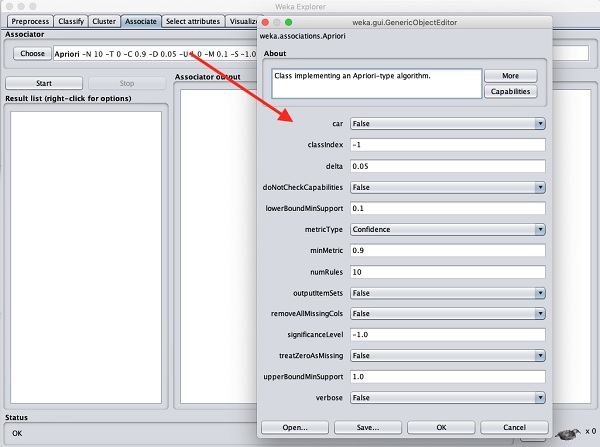
To set the parameters for the Apriori algorithm, click on its name, a window will pop up as shown below that allows you to set the parameters −

After you set the parameters, click the Start button. After a while you will see the results as shown in the screenshot below −

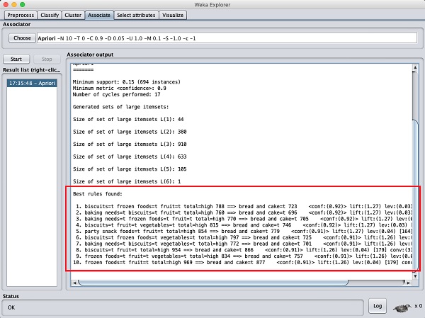
At the bottom, you will find the detected best rules of associations. This will help the supermarket in stocking their products in appropriate shelves.

Weka - Feature Selection

When a database contains a large number of attributes, there will be several attributes which do not become significant in the analysis that you are currently seeking. Thus, removing the unwanted attributes from the dataset becomes an important task in developing a good machine learning model.

You may examine the entire dataset visually and decide on the irrelevant attributes. This could be a huge task for databases containing a large number of attributes like the supermarket case that you saw in an earlier lesson. Fortunately, WEKA provides an automated tool for feature selection.

This chapter demonstrate this feature on a database containing a large number of attributes.

Loading Data

In the Preprocess tag of the WEKA explorer, select the labor.arff file for loading into the system. When you load the data, you will see the following screen −

Notice that there are 17 attributes. Our task is to create a reduced dataset by eliminating some of the attributes which are irrelevant to our analysis.

Features Extraction

Click on the Select attributesTAB.You will see the following screen −

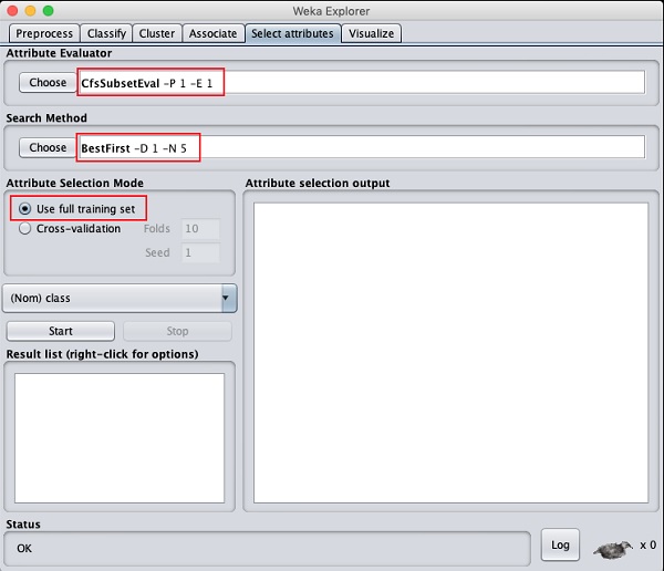
Under the Attribute Evaluator and Search Method, you will find several options. We will just use the defaults here. In the Attribute Selection Mode, use full training set option.

Click on the Start button to process the dataset. You will see the following output −

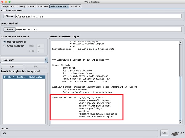
At the bottom of the result window, you will get the list of Selected attributes. To get the visual representation, right click on the result in the Result list.

The output is shown in the following screenshot −

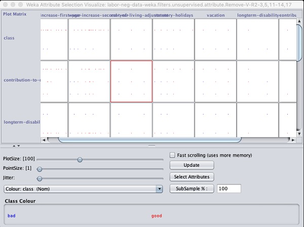
Clicking on any of the squares will give you the data plot for your further analysis. A typical data plot is shown below −

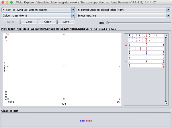
This is similar to the ones we have seen in the earlier chapters. Play around with the different options available to analyze the results.

What’s Next?

You have seen so far the power of WEKA in quickly developing machine learning models. What we used is a graphical tool called Explorer for developing these models. WEKA also provides a command line interface that gives you more power than provided in the explorer.

Clicking the Simple CLI button in the GUI Chooser application starts this command line interface which is shown in the screenshot below −

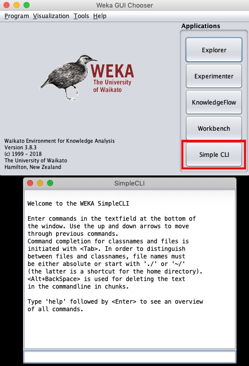
Type your commands in the input box at the bottom. You will be able to do all that you have done so far in the explorer plus much more. Refer to WEKA documentation (https://www.cs.waikato.ac.nz/ml/weka/documentation.html) for further details.

Lastly, WEKA is developed in Java and provides an interface to its API. So if you are a Java developer and keen to include WEKA ML implementations in your own Java projects, you can do so easily.

Conclusion

WEKA is a powerful tool for developing machine learning models. It provides implementation of several most widely used ML algorithms. Before these algorithms are applied to your dataset, it also allows you to preprocess the data. The types of algorithms that are supported are classified under Classify, Cluster, Associate, and Select attributes. The result at various stages of processing can be visualized with a beautiful and powerful visual representation. This makes it easier for a Data Scientist to quickly apply the various machine learning techniques on his dataset, compare the results and create the best model for the final use.