- Scikit Learn Tutorial
- Scikit Learn - Home
- Scikit Learn - Introduction
- Scikit Learn - Modelling Process
- Scikit Learn - Data Representation
- Scikit Learn - Estimator API
- Scikit Learn - Conventions
- Scikit Learn - Linear Modeling
- Scikit Learn - Extended Linear Modeling
- Stochastic Gradient Descent
- Scikit Learn - Support Vector Machines
- Scikit Learn - Anomaly Detection
- Scikit Learn - K-Nearest Neighbors
- Scikit Learn - KNN Learning
- Classification with Naïve Bayes
- Scikit Learn - Decision Trees
- Randomized Decision Trees
- Scikit Learn - Boosting Methods
- Scikit Learn - Clustering Methods
- Clustering Performance Evaluation
- Dimensionality Reduction using PCA
- Scikit Learn Useful Resources
- Scikit Learn - Quick Guide
- Scikit Learn - Useful Resources
- Scikit Learn - Discussion
Scikit Learn - Support Vector Machines
This chapter deals with a machine learning method termed as Support Vector Machines (SVMs).
Introduction
Support vector machines (SVMs) are powerful yet flexible supervised machine learning methods used for classification, regression, and, outliers’ detection. SVMs are very efficient in high dimensional spaces and generally are used in classification problems. SVMs are popular and memory efficient because they use a subset of training points in the decision function.
The main goal of SVMs is to divide the datasets into number of classes in order to find a maximum marginal hyperplane (MMH) which can be done in the following two steps −
Support Vector Machines will first generate hyperplanes iteratively that separates the classes in the best way.
After that it will choose the hyperplane that segregate the classes correctly.
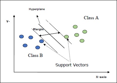
Some important concepts in SVM are as follows −
Support Vectors − They may be defined as the datapoints which are closest to the hyperplane. Support vectors help in deciding the separating line.
Hyperplane − The decision plane or space that divides set of objects having different classes.
Margin − The gap between two lines on the closet data points of different classes is called margin.
Following diagrams will give you an insight about these SVM concepts −
SVM in Scikit-learn supports both sparse and dense sample vectors as input.
Classification of SVM
Scikit-learn provides three classes namely SVC, NuSVC and LinearSVC which can perform multiclass-class classification.
SVC
It is C-support vector classification whose implementation is based on libsvm. The module used by scikit-learn is sklearn.svm.SVC. This class handles the multiclass support according to one-vs-one scheme.
Parameters
Followings table consist the parameters used by sklearn.svm.SVC class −
| Sr.No | Parameter & Description |
|---|---|
| 1 |
C − float, optional, default = 1.0 It is the penalty parameter of the error term. |
| 2 |
kernel − string, optional, default = ‘rbf’ This parameter specifies the type of kernel to be used in the algorithm. we can choose any one among, ‘linear’, ‘poly’, ‘rbf’, ‘sigmoid’, ‘precomputed’. The default value of kernel would be ‘rbf’. |
| 3 |
degree − int, optional, default = 3 It represents the degree of the ‘poly’ kernel function and will be ignored by all other kernels. |
| 4 |
gamma − {‘scale’, ‘auto’} or float, It is the kernel coefficient for kernels ‘rbf’, ‘poly’ and ‘sigmoid’. |
| 5 |
optinal default − = ‘scale’ If you choose default i.e. gamma = ‘scale’ then the value of gamma to be used by SVC is 1/(𝑛_𝑓𝑒𝑎𝑡𝑢𝑟𝑒𝑠∗𝑋.𝑣𝑎𝑟()). On the other hand, if gamma= ‘auto’, it uses 1/𝑛_𝑓𝑒𝑎𝑡𝑢𝑟𝑒𝑠. |
| 6 |
coef0 − float, optional, Default=0.0 An independent term in kernel function which is only significant in ‘poly’ and ‘sigmoid’. |
| 7 |
tol − float, optional, default = 1.e-3 This parameter represents the stopping criterion for iterations. |
| 8 |
shrinking − Boolean, optional, default = True This parameter represents that whether we want to use shrinking heuristic or not. |
| 9 |
verbose − Boolean, default: false It enables or disable verbose output. Its default value is false. |
| 10 |
probability − boolean, optional, default = true This parameter enables or disables probability estimates. The default value is false, but it must be enabled before we call fit. |
| 11 |
max_iter − int, optional, default = -1 As name suggest, it represents the maximum number of iterations within the solver. Value -1 means there is no limit on the number of iterations. |
| 12 |
cache_size − float, optional This parameter will specify the size of the kernel cache. The value will be in MB(MegaBytes). |
| 13 |
random_state − int, RandomState instance or None, optional, default = none This parameter represents the seed of the pseudo random number generated which is used while shuffling the data. Followings are the options −
|
| 14 |
class_weight − {dict, ‘balanced’}, optional This parameter will set the parameter C of class j to 𝑐𝑙𝑎𝑠𝑠_𝑤𝑒𝑖𝑔ℎ𝑡[𝑗]∗𝐶 for SVC. If we use the default option, it means all the classes are supposed to have weight one. On the other hand, if you choose class_weight:balanced, it will use the values of y to automatically adjust weights. |
| 15 |
decision_function_shape − ovo’, ‘ovr’, default = ‘ovr’ This parameter will decide whether the algorithm will return ‘ovr’ (one-vs-rest) decision function of shape as all other classifiers, or the original ovo(one-vs-one) decision function of libsvm. |
| 16 |
break_ties − boolean, optional, default = false True − The predict will break ties according to the confidence values of decision_function False − The predict will return the first class among the tied classes. |
Attributes
Followings table consist the attributes used by sklearn.svm.SVC class −
| Sr.No | Attributes & Description |
|---|---|
| 1 |
support_ − array-like, shape = [n_SV] It returns the indices of support vectors. |
| 2 |
support_vectors_ − array-like, shape = [n_SV, n_features] It returns the support vectors. |
| 3 |
n_support_ − array-like, dtype=int32, shape = [n_class] It represents the number of support vectors for each class. |
| 4 |
dual_coef_ − array, shape = [n_class-1,n_SV] These are the coefficient of the support vectors in the decision function. |
| 5 |
coef_ − array, shape = [n_class * (n_class-1)/2, n_features] This attribute, only available in case of linear kernel, provides the weight assigned to the features. |
| 6 |
intercept_ − array, shape = [n_class * (n_class-1)/2] It represents the independent term (constant) in decision function. |
| 7 |
fit_status_ − int The output would be 0 if it is correctly fitted. The output would be 1 if it is incorrectly fitted. |
| 8 |
classes_ − array of shape = [n_classes] It gives the labels of the classes. |
Implementation Example
Like other classifiers, SVC also has to be fitted with following two arrays −
An array X holding the training samples. It is of size [n_samples, n_features].
An array Y holding the target values i.e. class labels for the training samples. It is of size [n_samples].
Following Python script uses sklearn.svm.SVC class −
import numpy as np
X = np.array([[-1, -1], [-2, -1], [1, 1], [2, 1]])
y = np.array([1, 1, 2, 2])
from sklearn.svm import SVC
SVCClf = SVC(kernel = 'linear',gamma = 'scale', shrinking = False,)
SVCClf.fit(X, y)
Output
SVC(C = 1.0, cache_size = 200, class_weight = None, coef0 = 0.0,
   decision_function_shape = 'ovr', degree = 3, gamma = 'scale', kernel = 'linear',
   max_iter = -1, probability = False, random_state = None, shrinking = False,
   tol = 0.001, verbose = False)
Example
Now, once fitted, we can get the weight vector with the help of following python script −
SVCClf.coef_
Output
array([[0.5, 0.5]])
Example
Similarly, we can get the value of other attributes as follows −
SVCClf.predict([[-0.5,-0.8]])
Output
array([1])
Example
SVCClf.n_support_
Output
array([1, 1])
Example
SVCClf.support_vectors_
Output
array(
   [
      [-1., -1.],
      [ 1., 1.]
   ]
)
Example
SVCClf.support_
Output
array([0, 2])
Example
SVCClf.intercept_
Output
array([-0.])
Example
SVCClf.fit_status_
Output
0
NuSVC
NuSVC is Nu Support Vector Classification. It is another class provided by scikit-learn which can perform multi-class classification. It is like SVC but NuSVC accepts slightly different sets of parameters. The parameter which is different from SVC is as follows −
nu − float, optional, default = 0.5
It represents an upper bound on the fraction of training errors and a lower bound of the fraction of support vectors. Its value should be in the interval of (o,1].
Rest of the parameters and attributes are same as of SVC.
Implementation Example
We can implement the same example using sklearn.svm.NuSVC class also.
import numpy as np
X = np.array([[-1, -1], [-2, -1], [1, 1], [2, 1]])
y = np.array([1, 1, 2, 2])
from sklearn.svm import NuSVC
NuSVCClf = NuSVC(kernel = 'linear',gamma = 'scale', shrinking = False,)
NuSVCClf.fit(X, y)
Output
NuSVC(cache_size = 200, class_weight = None, coef0 = 0.0,
   decision_function_shape = 'ovr', degree = 3, gamma = 'scale', kernel = 'linear',
   max_iter = -1, nu = 0.5, probability = False, random_state = None,
   shrinking = False, tol = 0.001, verbose = False)
We can get the outputs of rest of the attributes as did in the case of SVC.
LinearSVC
It is Linear Support Vector Classification. It is similar to SVC having kernel = ‘linear’. The difference between them is that LinearSVC implemented in terms of liblinear while SVC is implemented in libsvm. That’s the reason LinearSVC has more flexibility in the choice of penalties and loss functions. It also scales better to large number of samples.
If we talk about its parameters and attributes then it does not support ‘kernel’ because it is assumed to be linear and it also lacks some of the attributes like support_, support_vectors_, n_support_, fit_status_ and, dual_coef_.
However, it supports penalty and loss parameters as follows −
penalty − string, L1 or L2(default = ‘L2’)
This parameter is used to specify the norm (L1 or L2) used in penalization (regularization).
loss − string, hinge, squared_hinge (default = squared_hinge)
It represents the loss function where ‘hinge’ is the standard SVM loss and ‘squared_hinge’ is the square of hinge loss.
Implementation Example
Following Python script uses sklearn.svm.LinearSVC class −
from sklearn.svm import LinearSVC
from sklearn.datasets import make_classification
X, y = make_classification(n_features = 4, random_state = 0)
LSVCClf = LinearSVC(dual = False, random_state = 0, penalty = 'l1',tol = 1e-5)
LSVCClf.fit(X, y)
Output
LinearSVC(C = 1.0, class_weight = None, dual = False, fit_intercept = True,
   intercept_scaling = 1, loss = 'squared_hinge', max_iter = 1000,
   multi_class = 'ovr', penalty = 'l1', random_state = 0, tol = 1e-05, verbose = 0)
Example
Now, once fitted, the model can predict new values as follows −
LSVCClf.predict([[0,0,0,0]])
Output
[1]
Example
For the above example, we can get the weight vector with the help of following python script −
LSVCClf.coef_
Output
[[0. 0. 0.91214955 0.22630686]]
Example
Similarly, we can get the value of intercept with the help of following python script −
LSVCClf.intercept_
Output
[0.26860518]
Regression with SVM
As discussed earlier, SVM is used for both classification and regression problems. Scikit-learn’s method of Support Vector Classification (SVC) can be extended to solve regression problems as well. That extended method is called Support Vector Regression (SVR).
Basic similarity between SVM and SVR
The model created by SVC depends only on a subset of training data. Why? Because the cost function for building the model doesn’t care about training data points that lie outside the margin.
Whereas, the model produced by SVR (Support Vector Regression) also only depends on a subset of the training data. Why? Because the cost function for building the model ignores any training data points close to the model prediction.
Scikit-learn provides three classes namely SVR, NuSVR and LinearSVR as three different implementations of SVR.
SVR
It is Epsilon-support vector regression whose implementation is based on libsvm. As opposite to SVC There are two free parameters in the model namely ‘C’ and ‘epsilon’.
epsilon − float, optional, default = 0.1
It represents the epsilon in the epsilon-SVR model, and specifies the epsilon-tube within which no penalty is associated in the training loss function with points predicted within a distance epsilon from the actual value.
Rest of the parameters and attributes are similar as we used in SVC.
Implementation Example
Following Python script uses sklearn.svm.SVR class −
from sklearn import svm
X = [[1, 1], [2, 2]]
y = [1, 2]
SVRReg = svm.SVR(kernel = ’linear’, gamma = ’auto’)
SVRReg.fit(X, y)
Output
SVR(C = 1.0, cache_size = 200, coef0 = 0.0, degree = 3, epsilon = 0.1, gamma = 'auto',
   kernel = 'linear', max_iter = -1, shrinking = True, tol = 0.001, verbose = False)
Example
Now, once fitted, we can get the weight vector with the help of following python script −
SVRReg.coef_
Output
array([[0.4, 0.4]])
Example
Similarly, we can get the value of other attributes as follows −
SVRReg.predict([[1,1]])
Output
array([1.1])
Similarly, we can get the values of other attributes as well.
NuSVR
NuSVR is Nu Support Vector Regression. It is like NuSVC, but NuSVR uses a parameter nu to control the number of support vectors. And moreover, unlike NuSVC where nu replaced C parameter, here it replaces epsilon.
Implementation Example
Following Python script uses sklearn.svm.SVR class −
from sklearn.svm import NuSVR
import numpy as np
n_samples, n_features = 20, 15
np.random.seed(0)
y = np.random.randn(n_samples)
X = np.random.randn(n_samples, n_features)
NuSVRReg = NuSVR(kernel = 'linear', gamma = 'auto',C = 1.0, nu = 0.1)^M
NuSVRReg.fit(X, y)
Output
NuSVR(C = 1.0, cache_size = 200, coef0 = 0.0, degree = 3, gamma = 'auto',
   kernel = 'linear', max_iter = -1, nu = 0.1, shrinking = True, tol = 0.001,
   verbose = False)
Example
Now, once fitted, we can get the weight vector with the help of following python script −
NuSVRReg.coef_
Output
array(
   [
      [-0.14904483, 0.04596145, 0.22605216, -0.08125403, 0.06564533,
      0.01104285, 0.04068767, 0.2918337 , -0.13473211, 0.36006765,
      -0.2185713 , -0.31836476, -0.03048429, 0.16102126, -0.29317051]
   ]
)
Similarly, we can get the value of other attributes as well.
LinearSVR
It is Linear Support Vector Regression. It is similar to SVR having kernel = ‘linear’. The difference between them is that LinearSVR implemented in terms of liblinear, while SVC implemented in libsvm. That’s the reason LinearSVR has more flexibility in the choice of penalties and loss functions. It also scales better to large number of samples.
If we talk about its parameters and attributes then it does not support ‘kernel’ because it is assumed to be linear and it also lacks some of the attributes like support_, support_vectors_, n_support_, fit_status_ and, dual_coef_.
However, it supports ‘loss’ parameters as follows −
loss − string, optional, default = ‘epsilon_insensitive’
It represents the loss function where epsilon_insensitive loss is the L1 loss and the squared epsilon-insensitive loss is the L2 loss.
Implementation Example
Following Python script uses sklearn.svm.LinearSVR class −
from sklearn.svm import LinearSVR
from sklearn.datasets import make_regression
X, y = make_regression(n_features = 4, random_state = 0)
LSVRReg = LinearSVR(dual = False, random_state = 0,
loss = 'squared_epsilon_insensitive',tol = 1e-5)
LSVRReg.fit(X, y)
Output
LinearSVR(
   C=1.0, dual=False, epsilon=0.0, fit_intercept=True,
   intercept_scaling=1.0, loss='squared_epsilon_insensitive',
   max_iter=1000, random_state=0, tol=1e-05, verbose=0
)
Example
Now, once fitted, the model can predict new values as follows −
LSRReg.predict([[0,0,0,0]])
Output
array([-0.01041416])
Example
For the above example, we can get the weight vector with the help of following python script −
LSRReg.coef_
Output
array([20.47354746, 34.08619401, 67.23189022, 87.47017787])
Example
Similarly, we can get the value of intercept with the help of following python script −
LSRReg.intercept_
Output
array([-0.01041416])