- Scikit Learn Tutorial
- Scikit Learn - Home
- Scikit Learn - Introduction
- Scikit Learn - Modelling Process
- Scikit Learn - Data Representation
- Scikit Learn - Estimator API
- Scikit Learn - Conventions
- Scikit Learn - Linear Modeling
- Scikit Learn - Extended Linear Modeling
- Stochastic Gradient Descent
- Scikit Learn - Support Vector Machines
- Scikit Learn - Anomaly Detection
- Scikit Learn - K-Nearest Neighbors
- Scikit Learn - KNN Learning
- Classification with Naïve Bayes
- Scikit Learn - Decision Trees
- Randomized Decision Trees
- Scikit Learn - Boosting Methods
- Scikit Learn - Clustering Methods
- Clustering Performance Evaluation
- Dimensionality Reduction using PCA
- Scikit Learn Useful Resources
- Scikit Learn - Quick Guide
- Scikit Learn - Useful Resources
- Scikit Learn - Discussion
Scikit Learn - Quick Guide
Scikit Learn - Introduction
In this chapter, we will understand what is Scikit-Learn or Sklearn, origin of Scikit-Learn and some other related topics such as communities and contributors responsible for development and maintenance of Scikit-Learn, its prerequisites, installation and its features.
What is Scikit-Learn (Sklearn)
Scikit-learn (Sklearn) is the most useful and robust library for machine learning in Python. It provides a selection of efficient tools for machine learning and statistical modeling including classification, regression, clustering and dimensionality reduction via a consistence interface in Python. This library, which is largely written in Python, is built upon NumPy, SciPy and Matplotlib.
Origin of Scikit-Learn
It was originally called scikits.learn and was initially developed by David Cournapeau as a Google summer of code project in 2007. Later, in 2010, Fabian Pedregosa, Gael Varoquaux, Alexandre Gramfort, and Vincent Michel, from FIRCA (French Institute for Research in Computer Science and Automation), took this project at another level and made the first public release (v0.1 beta) on 1st Feb. 2010.
Let’s have a look at its version history −
May 2019: scikit-learn 0.21.0
March 2019: scikit-learn 0.20.3
December 2018: scikit-learn 0.20.2
November 2018: scikit-learn 0.20.1
September 2018: scikit-learn 0.20.0
July 2018: scikit-learn 0.19.2
July 2017: scikit-learn 0.19.0
September 2016. scikit-learn 0.18.0
November 2015. scikit-learn 0.17.0
March 2015. scikit-learn 0.16.0
July 2014. scikit-learn 0.15.0
August 2013. scikit-learn 0.14
Community & contributors
Scikit-learn is a community effort and anyone can contribute to it. This project is hosted on https://github.com/scikit-learn/scikit-learn. Following people are currently the core contributors to Sklearn’s development and maintenance −
Joris Van den Bossche (Data Scientist)
Thomas J Fan (Software Developer)
Alexandre Gramfort (Machine Learning Researcher)
Olivier Grisel (Machine Learning Expert)
Nicolas Hug (Associate Research Scientist)
Andreas Mueller (Machine Learning Scientist)
Hanmin Qin (Software Engineer)
Adrin Jalali (Open Source Developer)
Nelle Varoquaux (Data Science Researcher)
Roman Yurchak (Data Scientist)
Various organisations like Booking.com, JP Morgan, Evernote, Inria, AWeber, Spotify and many more are using Sklearn.
Prerequisites
Before we start using scikit-learn latest release, we require the following −
Python (>=3.5)
NumPy (>= 1.11.0)
Scipy (>= 0.17.0)li
Joblib (>= 0.11)
Matplotlib (>= 1.5.1) is required for Sklearn plotting capabilities.
Pandas (>= 0.18.0) is required for some of the scikit-learn examples using data structure and analysis.
Installation
If you already installed NumPy and Scipy, following are the two easiest ways to install scikit-learn −
Using pip
Following command can be used to install scikit-learn via pip −
pip install -U scikit-learn
Using conda
Following command can be used to install scikit-learn via conda −
conda install scikit-learn
On the other hand, if NumPy and Scipy is not yet installed on your Python workstation then, you can install them by using either pip or conda.
Another option to use scikit-learn is to use Python distributions like Canopy and Anaconda because they both ship the latest version of scikit-learn.
Features
Rather than focusing on loading, manipulating and summarising data, Scikit-learn library is focused on modeling the data. Some of the most popular groups of models provided by Sklearn are as follows −
Supervised Learning algorithms − Almost all the popular supervised learning algorithms, like Linear Regression, Support Vector Machine (SVM), Decision Tree etc., are the part of scikit-learn.
Unsupervised Learning algorithms − On the other hand, it also has all the popular unsupervised learning algorithms from clustering, factor analysis, PCA (Principal Component Analysis) to unsupervised neural networks.
Clustering − This model is used for grouping unlabeled data.
Cross Validation − It is used to check the accuracy of supervised models on unseen data.
Dimensionality Reduction − It is used for reducing the number of attributes in data which can be further used for summarisation, visualisation and feature selection.
Ensemble methods − As name suggest, it is used for combining the predictions of multiple supervised models.
Feature extraction − It is used to extract the features from data to define the attributes in image and text data.
Feature selection − It is used to identify useful attributes to create supervised models.
Open Source − It is open source library and also commercially usable under BSD license.
Scikit Learn - Modelling Process
This chapter deals with the modelling process involved in Sklearn. Let us understand about the same in detail and begin with dataset loading.
Dataset Loading
A collection of data is called dataset. It is having the following two components −
Features − The variables of data are called its features. They are also known as predictors, inputs or attributes.
Feature matrix − It is the collection of features, in case there are more than one.
Feature Names − It is the list of all the names of the features.
Response − It is the output variable that basically depends upon the feature variables. They are also known as target, label or output.
Response Vector − It is used to represent response column. Generally, we have just one response column.
Target Names − It represent the possible values taken by a response vector.
Scikit-learn have few example datasets like iris and digits for classification and the Boston house prices for regression.
Example
Following is an example to load iris dataset −
from sklearn.datasets import load_iris
iris = load_iris()
X = iris.data
y = iris.target
feature_names = iris.feature_names
target_names = iris.target_names
print("Feature names:", feature_names)
print("Target names:", target_names)
print("\nFirst 10 rows of X:\n", X[:10])
Output
Feature names: ['sepal length (cm)', 'sepal width (cm)', 'petal length (cm)', 'petal width (cm)']
Target names: ['setosa' 'versicolor' 'virginica']
First 10 rows of X:
[
   [5.1 3.5 1.4 0.2]
   [4.9 3. 1.4 0.2]
   [4.7 3.2 1.3 0.2]
   [4.6 3.1 1.5 0.2]
   [5. 3.6 1.4 0.2]
   [5.4 3.9 1.7 0.4]
   [4.6 3.4 1.4 0.3]
   [5. 3.4 1.5 0.2]
   [4.4 2.9 1.4 0.2]
   [4.9 3.1 1.5 0.1]
]
Splitting the dataset
To check the accuracy of our model, we can split the dataset into two pieces-a training set and a testing set. Use the training set to train the model and testing set to test the model. After that, we can evaluate how well our model did.
Example
The following example will split the data into 70:30 ratio, i.e. 70% data will be used as training data and 30% will be used as testing data. The dataset is iris dataset as in above example.
from sklearn.datasets import load_iris
iris = load_iris()

X = iris.data
y = iris.target

from sklearn.model_selection import train_test_split

X_train, X_test, y_train, y_test = train_test_split(
   X, y, test_size = 0.3, random_state = 1
)

print(X_train.shape)
print(X_test.shape)

print(y_train.shape)
print(y_test.shape)
Output
(105, 4)
(45, 4)
(105,)
(45,)
As seen in the example above, it uses train_test_split() function of scikit-learn to split the dataset. This function has the following arguments −
X, y − Here, X is the feature matrix and y is the response vector, which need to be split.
test_size − This represents the ratio of test data to the total given data. As in the above example, we are setting test_data = 0.3 for 150 rows of X. It will produce test data of 150*0.3 = 45 rows.
random_size − It is used to guarantee that the split will always be the same. This is useful in the situations where you want reproducible results.
Train the Model
Next, we can use our dataset to train some prediction-model. As discussed, scikit-learn has wide range of Machine Learning (ML) algorithms which have a consistent interface for fitting, predicting accuracy, recall etc.
Example
In the example below, we are going to use KNN (K nearest neighbors) classifier. Don’t go into the details of KNN algorithms, as there will be a separate chapter for that. This example is used to make you understand the implementation part only.
from sklearn.datasets import load_iris
iris = load_iris()
X = iris.data
y = iris.target
from sklearn.model_selection import train_test_split
X_train, X_test, y_train, y_test = train_test_split(
   X, y, test_size = 0.4, random_state=1
)
from sklearn.neighbors import KNeighborsClassifier
from sklearn import metrics
classifier_knn = KNeighborsClassifier(n_neighbors = 3)
classifier_knn.fit(X_train, y_train)
y_pred = classifier_knn.predict(X_test)
# Finding accuracy by comparing actual response values(y_test)with predicted response value(y_pred)
print("Accuracy:", metrics.accuracy_score(y_test, y_pred))
# Providing sample data and the model will make prediction out of that data

sample = [[5, 5, 3, 2], [2, 4, 3, 5]]
preds = classifier_knn.predict(sample)
pred_species = [iris.target_names[p] for p in preds] print("Predictions:", pred_species)
Output
Accuracy: 0.9833333333333333
Predictions: ['versicolor', 'virginica']
Model Persistence
Once you train the model, it is desirable that the model should be persist for future use so that we do not need to retrain it again and again. It can be done with the help of dump and load features of joblib package.
Consider the example below in which we will be saving the above trained model (classifier_knn) for future use −
from sklearn.externals import joblib
joblib.dump(classifier_knn, 'iris_classifier_knn.joblib')
The above code will save the model into file named iris_classifier_knn.joblib. Now, the object can be reloaded from the file with the help of following code −
joblib.load('iris_classifier_knn.joblib')
Preprocessing the Data
As we are dealing with lots of data and that data is in raw form, before inputting that data to machine learning algorithms, we need to convert it into meaningful data. This process is called preprocessing the data. Scikit-learn has package named preprocessing for this purpose. The preprocessing package has the following techniques −
Binarisation
This preprocessing technique is used when we need to convert our numerical values into Boolean values.
Example
import numpy as np
from sklearn import preprocessing
Input_data = np.array(
   [2.1, -1.9, 5.5],
   [-1.5, 2.4, 3.5],
   [0.5, -7.9, 5.6],
   [5.9, 2.3, -5.8]]
)
data_binarized = preprocessing.Binarizer(threshold=0.5).transform(input_data)
print("\nBinarized data:\n", data_binarized)
In the above example, we used threshold value = 0.5 and that is why, all the values above 0.5 would be converted to 1, and all the values below 0.5 would be converted to 0.
Output
Binarized data:
[
   [ 1. 0. 1.]
   [ 0. 1. 1.]
   [ 0. 0. 1.]
   [ 1. 1. 0.]
]
Mean Removal
This technique is used to eliminate the mean from feature vector so that every feature centered on zero.
Example
import numpy as np
from sklearn import preprocessing
Input_data = np.array(
   [2.1, -1.9, 5.5],
   [-1.5, 2.4, 3.5],
   [0.5, -7.9, 5.6],
   [5.9, 2.3, -5.8]]
)

#displaying the mean and the standard deviation of the input data
print("Mean =", input_data.mean(axis=0))
print("Stddeviation = ", input_data.std(axis=0))
#Removing the mean and the standard deviation of the input data

data_scaled = preprocessing.scale(input_data)
print("Mean_removed =", data_scaled.mean(axis=0))
print("Stddeviation_removed =", data_scaled.std(axis=0))
Output
Mean = [ 1.75 -1.275 2.2 ]
Stddeviation = [ 2.71431391 4.20022321 4.69414529]
Mean_removed = [ 1.11022302e-16 0.00000000e+00 0.00000000e+00]
Stddeviation_removed = [ 1. 1. 1.]
Scaling
We use this preprocessing technique for scaling the feature vectors. Scaling of feature vectors is important, because the features should not be synthetically large or small.
Example
import numpy as np
from sklearn import preprocessing
Input_data = np.array(
   [
      [2.1, -1.9, 5.5],
      [-1.5, 2.4, 3.5],
      [0.5, -7.9, 5.6],
      [5.9, 2.3, -5.8]
   ]
)
data_scaler_minmax = preprocessing.MinMaxScaler(feature_range=(0,1))
data_scaled_minmax = data_scaler_minmax.fit_transform(input_data)
print ("\nMin max scaled data:\n", data_scaled_minmax)
Output
Min max scaled data:
[
   [ 0.48648649 0.58252427 0.99122807]
   [ 0. 1. 0.81578947]
   [ 0.27027027 0. 1. ]
   [ 1. 0.99029126 0. ]
]
Normalisation
We use this preprocessing technique for modifying the feature vectors. Normalisation of feature vectors is necessary so that the feature vectors can be measured at common scale. There are two types of normalisation as follows −
L1 Normalisation
It is also called Least Absolute Deviations. It modifies the value in such a manner that the sum of the absolute values remains always up to 1 in each row. Following example shows the implementation of L1 normalisation on input data.
Example
import numpy as np
from sklearn import preprocessing
Input_data = np.array(
   [
      [2.1, -1.9, 5.5],
      [-1.5, 2.4, 3.5],
      [0.5, -7.9, 5.6],
      [5.9, 2.3, -5.8]
   ]
)
data_normalized_l1 = preprocessing.normalize(input_data, norm='l1')
print("\nL1 normalized data:\n", data_normalized_l1)
Output
L1 normalized data:
[
   [ 0.22105263 -0.2 0.57894737]
   [-0.2027027 0.32432432 0.47297297]
   [ 0.03571429 -0.56428571 0.4 ]
   [ 0.42142857 0.16428571 -0.41428571]
]
L2 Normalisation
Also called Least Squares. It modifies the value in such a manner that the sum of the squares remains always up to 1 in each row. Following example shows the implementation of L2 normalisation on input data.
Example
import numpy as np
from sklearn import preprocessing
Input_data = np.array(
   [
      [2.1, -1.9, 5.5],
      [-1.5, 2.4, 3.5],
      [0.5, -7.9, 5.6],
      [5.9, 2.3, -5.8]
   ]
)
data_normalized_l2 = preprocessing.normalize(input_data, norm='l2')
print("\nL1 normalized data:\n", data_normalized_l2)
Output
L2 normalized data:
[
   [ 0.33946114 -0.30713151 0.88906489]
   [-0.33325106 0.53320169 0.7775858 ]
   [ 0.05156558 -0.81473612 0.57753446]
   [ 0.68706914 0.26784051 -0.6754239 ]
]
Scikit Learn - Data Representation
As we know that machine learning is about to create model from data. For this purpose, computer must understand the data first. Next, we are going to discuss various ways to represent the data in order to be understood by computer −
Data as table
The best way to represent data in Scikit-learn is in the form of tables. A table represents a 2-D grid of data where rows represent the individual elements of the dataset and the columns represents the quantities related to those individual elements.
Example
With the example given below, we can download iris dataset in the form of a Pandas DataFrame with the help of python seaborn library.
import seaborn as sns
iris = sns.load_dataset('iris')
iris.head()
Output
sepal_length sepal_width petal_length petal_width  species
0        5.1      3.5         1.4             0.2   setosa
1        4.9      3.0         1.4             0.2   setosa
2        4.7      3.2         1.3             0.2   setosa
3        4.6      3.1         1.5             0.2   setosa
4        5.0      3.6         1.4             0.2   setosa
From above output, we can see that each row of the data represents a single observed flower and the number of rows represents the total number of flowers in the dataset. Generally, we refer the rows of the matrix as samples.
On the other hand, each column of the data represents a quantitative information describing each sample. Generally, we refer the columns of the matrix as features.
Data as Feature Matrix
Features matrix may be defined as the table layout where information can be thought of as a 2-D matrix. It is stored in a variable named X and assumed to be two dimensional with shape [n_samples, n_features]. Mostly, it is contained in a NumPy array or a Pandas DataFrame. As told earlier, the samples always represent the individual objects described by the dataset and the features represents the distinct observations that describe each sample in a quantitative manner.
Data as Target array
Along with Features matrix, denoted by X, we also have target array. It is also called label. It is denoted by y. The label or target array is usually one-dimensional having length n_samples. It is generally contained in NumPy array or Pandas Series. Target array may have both the values, continuous numerical values and discrete values.
How target array differs from feature columns?
We can distinguish both by one point that the target array is usually the quantity we want to predict from the data i.e. in statistical terms it is the dependent variable.
Example
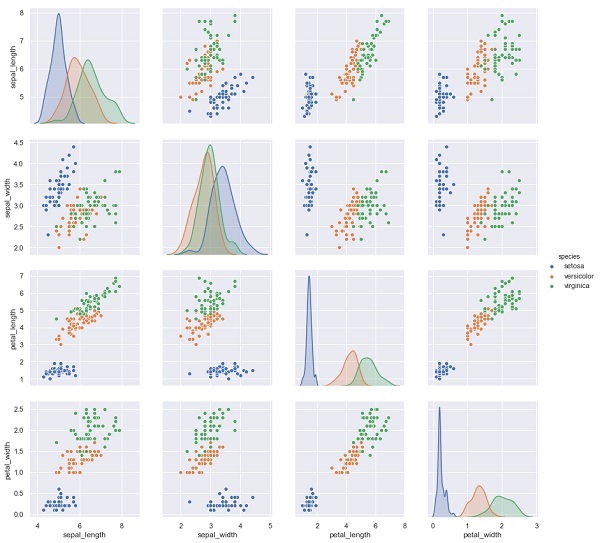
In the example below, from iris dataset we predict the species of flower based on the other measurements. In this case, the Species column would be considered as the feature.
import seaborn as sns
iris = sns.load_dataset('iris')
%matplotlib inline
import seaborn as sns; sns.set()
sns.pairplot(iris, hue='species', height=3);
Output
X_iris = iris.drop('species', axis=1)
X_iris.shape
y_iris = iris['species']
y_iris.shape
Output
(150,4)
(150,)
Scikit Learn - Estimator API
In this chapter, we will learn about Estimator API (application programming interface). Let us begin by understanding what is an Estimator API.
What is Estimator API
It is one of the main APIs implemented by Scikit-learn. It provides a consistent interface for a wide range of ML applications that’s why all machine learning algorithms in Scikit-Learn are implemented via Estimator API. The object that learns from the data (fitting the data) is an estimator. It can be used with any of the algorithms like classification, regression, clustering or even with a transformer, that extracts useful features from raw data.
For fitting the data, all estimator objects expose a fit method that takes a dataset shown as follows −
estimator.fit(data)
Next, all the parameters of an estimator can be set, as follows, when it is instantiated by the corresponding attribute.
estimator = Estimator (param1=1, param2=2)
estimator.param1
The output of the above would be 1.
Once data is fitted with an estimator, parameters are estimated from the data at hand. Now, all the estimated parameters will be the attributes of the estimator object ending by an underscore as follows −
estimator.estimated_param_
Use of Estimator API
Main uses of estimators are as follows −
Estimation and decoding of a model
Estimator object is used for estimation and decoding of a model. Furthermore, the model is estimated as a deterministic function of the following −
The parameters which are provided in object construction.
The global random state (numpy.random) if the estimator’s random_state parameter is set to none.
Any data passed to the most recent call to fit, fit_transform, or fit_predict.
Any data passed in a sequence of calls to partial_fit.
Mapping non-rectangular data representation into rectangular data
It maps a non-rectangular data representation into rectangular data. In simple words, it takes input where each sample is not represented as an array-like object of fixed length, and producing an array-like object of features for each sample.
Distinction between core and outlying samples
It models the distinction between core and outlying samples by using following methods −
fit
fit_predict if transductive
predict if inductive
Guiding Principles
While designing the Scikit-Learn API, following guiding principles kept in mind −
Consistency
This principle states that all the objects should share a common interface drawn from a limited set of methods. The documentation should also be consistent.
Limited object hierarchy
This guiding principle says −
Algorithms should be represented by Python classes
Datasets should be represented in standard format like NumPy arrays, Pandas DataFrames, SciPy sparse matrix.
Parameters names should use standard Python strings.
Composition
As we know that, ML algorithms can be expressed as the sequence of many fundamental algorithms. Scikit-learn makes use of these fundamental algorithms whenever needed.
Sensible defaults
According to this principle, the Scikit-learn library defines an appropriate default value whenever ML models require user-specified parameters.
Inspection
As per this guiding principle, every specified parameter value is exposed as pubic attributes.
Steps in using Estimator API
Followings are the steps in using the Scikit-Learn estimator API −
Step 1: Choose a class of model
In this first step, we need to choose a class of model. It can be done by importing the appropriate Estimator class from Scikit-learn.
Step 2: Choose model hyperparameters
In this step, we need to choose class model hyperparameters. It can be done by instantiating the class with desired values.
Step 3: Arranging the data
Next, we need to arrange the data into features matrix (X) and target vector(y).
Step 4: Model Fitting
Now, we need to fit the model to your data. It can be done by calling fit() method of the model instance.
Step 5: Applying the model
After fitting the model, we can apply it to new data. For supervised learning, use predict() method to predict the labels for unknown data. While for unsupervised learning, use predict() or transform() to infer properties of the data.
Supervised Learning Example
Here, as an example of this process we are taking common case of fitting a line to (x,y) data i.e. simple linear regression.
First, we need to load the dataset, we are using iris dataset −
Example
import seaborn as sns
iris = sns.load_dataset('iris')
X_iris = iris.drop('species', axis = 1)
X_iris.shape
Output
(150, 4)
Example
y_iris = iris['species']
y_iris.shape
Output
(150,)
Example
Now, for this regression example, we are going to use the following sample data −
%matplotlib inline
import matplotlib.pyplot as plt
import numpy as np
rng = np.random.RandomState(35)
x = 10*rng.rand(40)
y = 2*x-1+rng.randn(40)
plt.scatter(x,y);
Output
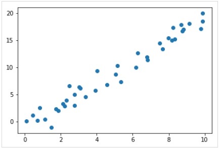
So, we have the above data for our linear regression example.
Now, with this data, we can apply the above-mentioned steps.
Choose a class of model
Here, to compute a simple linear regression model, we need to import the linear regression class as follows −
from sklearn.linear_model import LinearRegression
Choose model hyperparameters
Once we choose a class of model, we need to make some important choices which are often represented as hyperparameters, or the parameters that must set before the model is fit to data. Here, for this example of linear regression, we would like to fit the intercept by using the fit_intercept hyperparameter as follows −
Example
model = LinearRegression(fit_intercept = True)
model
Output
LinearRegression(copy_X = True, fit_intercept = True, n_jobs = None, normalize = False)
Arranging the data
Now, as we know that our target variable y is in correct form i.e. a length n_samples array of 1-D. But, we need to reshape the feature matrix X to make it a matrix of size [n_samples, n_features]. It can be done as follows −
Example
X = x[:, np.newaxis]
X.shape
Output
(40, 1)
Model fitting
Once, we arrange the data, it is time to fit the model i.e. to apply our model to data. This can be done with the help of fit() method as follows −
Example
model.fit(X, y)
Output
LinearRegression(copy_X = True, fit_intercept = True, n_jobs = None,normalize = False)
In Scikit-learn, the fit() process have some trailing underscores.
For this example, the below parameter shows the slope of the simple linear fit of the data −
Example
model.coef_
Output
array([1.99839352])
The below parameter represents the intercept of the simple linear fit to the data −
Example
model.intercept_
Output
-0.9895459457775022
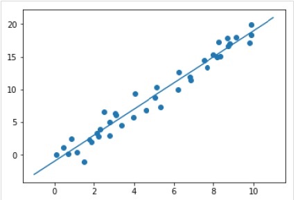
Applying the model to new data
After training the model, we can apply it to new data. As the main task of supervised machine learning is to evaluate the model based on new data that is not the part of the training set. It can be done with the help of predict() method as follows −
Example
xfit = np.linspace(-1, 11)
Xfit = xfit[:, np.newaxis]
yfit = model.predict(Xfit)
plt.scatter(x, y)
plt.plot(xfit, yfit);
Output
Complete working/executable example
%matplotlib inline
import matplotlib.pyplot as plt
import numpy as np
import seaborn as sns

iris = sns.load_dataset('iris')
X_iris = iris.drop('species', axis = 1)
X_iris.shape
y_iris = iris['species']
y_iris.shape

rng = np.random.RandomState(35)
x = 10*rng.rand(40)
y = 2*x-1+rng.randn(40)
plt.scatter(x,y);
from sklearn.linear_model import LinearRegression
model = LinearRegression(fit_intercept=True)
model
X = x[:, np.newaxis]
X.shape

model.fit(X, y)
model.coef_
model.intercept_

xfit = np.linspace(-1, 11)
Xfit = xfit[:, np.newaxis]
yfit = model.predict(Xfit)
plt.scatter(x, y)
plt.plot(xfit, yfit);
Unsupervised Learning Example
Here, as an example of this process we are taking common case of reducing the dimensionality of the Iris dataset so that we can visualize it more easily. For this example, we are going to use principal component analysis (PCA), a fast-linear dimensionality reduction technique.
Like the above given example, we can load and plot the random data from iris dataset. After that we can follow the steps as below −
Choose a class of model
from sklearn.decomposition import PCA
Choose model hyperparameters
Example
model = PCA(n_components=2)
model
Output
PCA(copy = True, iterated_power = 'auto', n_components = 2, random_state = None,
   svd_solver = 'auto', tol = 0.0, whiten = False)
Model fitting
Example
model.fit(X_iris)
Output
PCA(copy = True, iterated_power = 'auto', n_components = 2, random_state = None,
   svd_solver = 'auto', tol = 0.0, whiten = False)
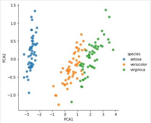
Transform the data to two-dimensional
Example
X_2D = model.transform(X_iris)
Now, we can plot the result as follows −
Output
iris['PCA1'] = X_2D[:, 0]
iris['PCA2'] = X_2D[:, 1]
sns.lmplot("PCA1", "PCA2", hue = 'species', data = iris, fit_reg = False);
Output
Complete working/executable example
%matplotlib inline
import matplotlib.pyplot as plt
import numpy as np
import seaborn as sns

iris = sns.load_dataset('iris')
X_iris = iris.drop('species', axis = 1)
X_iris.shape
y_iris = iris['species']
y_iris.shape
rng = np.random.RandomState(35)
x = 10*rng.rand(40)
y = 2*x-1+rng.randn(40)
plt.scatter(x,y);
from sklearn.decomposition import PCA

model = PCA(n_components=2)
model
model.fit(X_iris)
X_2D = model.transform(X_iris)
iris['PCA1'] = X_2D[:, 0]
iris['PCA2'] = X_2D[:, 1]
sns.lmplot("PCA1", "PCA2", hue='species', data=iris, fit_reg=False);
Scikit Learn - Conventions
Scikit-learn’s objects share a uniform basic API that consists of the following three complementary interfaces −
Estimator interface − It is for building and fitting the models.
Predictor interface − It is for making predictions.
Transformer interface − It is for converting data.
The APIs adopt simple conventions and the design choices have been guided in a manner to avoid the proliferation of framework code.
Purpose of Conventions
The purpose of conventions is to make sure that the API stick to the following broad principles −
Consistency − All the objects whether they are basic, or composite must share a consistent interface which further composed of a limited set of methods.
Inspection − Constructor parameters and parameters values determined by learning algorithm should be stored and exposed as public attributes.
Non-proliferation of classes − Datasets should be represented as NumPy arrays or Scipy sparse matrix whereas hyper-parameters names and values should be represented as standard Python strings to avoid the proliferation of framework code.
Composition − The algorithms whether they are expressible as sequences or combinations of transformations to the data or naturally viewed as meta-algorithms parameterized on other algorithms, should be implemented and composed from existing building blocks.
Sensible defaults − In scikit-learn whenever an operation requires a user-defined parameter, an appropriate default value is defined. This default value should cause the operation to be performed in a sensible way, for example, giving a base-line solution for the task at hand.
Various Conventions
The conventions available in Sklearn are explained below −
Type casting
It states that the input should be cast to float64. In the following example, in which sklearn.random_projection module used to reduce the dimensionality of the data, will explain it −
Example
import numpy as np
from sklearn import random_projection
rannge = np.random.RandomState(0)
X = range.rand(10,2000)
X = np.array(X, dtype = 'float32')
X.dtype
Transformer_data = random_projection.GaussianRandomProjection()
X_new = transformer.fit_transform(X)
X_new.dtype
Output
dtype('float32')
dtype('float64')
In the above example, we can see that X is float32 which is cast to float64 by fit_transform(X).
Refitting & Updating Parameters
Hyper-parameters of an estimator can be updated and refitted after it has been constructed via the set_params() method. Let’s see the following example to understand it −
Example
import numpy as np
from sklearn.datasets import load_iris
from sklearn.svm import SVC
X, y = load_iris(return_X_y = True)
clf = SVC()
clf.set_params(kernel = 'linear').fit(X, y)
clf.predict(X[:5])
Output
array([0, 0, 0, 0, 0])
Once the estimator has been constructed, above code will change the default kernel rbf to linear via SVC.set_params().
Now, the following code will change back the kernel to rbf to refit the estimator and to make a second prediction.
Example
clf.set_params(kernel = 'rbf', gamma = 'scale').fit(X, y)
clf.predict(X[:5])
Output
array([0, 0, 0, 0, 0])
Complete code
The following is the complete executable program −
import numpy as np
from sklearn.datasets import load_iris
from sklearn.svm import SVC
X, y = load_iris(return_X_y = True)
clf = SVC()
clf.set_params(kernel = 'linear').fit(X, y)
clf.predict(X[:5])
clf.set_params(kernel = 'rbf', gamma = 'scale').fit(X, y)
clf.predict(X[:5])
Multiclass & Multilabel fitting
In case of multiclass fitting, both learning and the prediction tasks are dependent on the format of the target data fit upon. The module used is sklearn.multiclass. Check the example below, where multiclass classifier is fit on a 1d array.
Example
from sklearn.svm import SVC
from sklearn.multiclass import OneVsRestClassifier
from sklearn.preprocessing import LabelBinarizer
X = [[1, 2], [3, 4], [4, 5], [5, 2], [1, 1]]
y = [0, 0, 1, 1, 2]
classif = OneVsRestClassifier(estimator = SVC(gamma = 'scale',random_state = 0))
classif.fit(X, y).predict(X)
Output
array([0, 0, 1, 1, 2])
In the above example, classifier is fit on one dimensional array of multiclass labels and the predict() method hence provides corresponding multiclass prediction. But on the other hand, it is also possible to fit upon a two-dimensional array of binary label indicators as follows −
Example
from sklearn.svm import SVC
from sklearn.multiclass import OneVsRestClassifier
from sklearn.preprocessing import LabelBinarizer
X = [[1, 2], [3, 4], [4, 5], [5, 2], [1, 1]]
y = LabelBinarizer().fit_transform(y)
classif.fit(X, y).predict(X)
Output
array(
   [
      [0, 0, 0],
      [0, 0, 0],
      [0, 1, 0],
      [0, 1, 0],
      [0, 0, 0]
   ]
)
Similarly, in case of multilabel fitting, an instance can be assigned multiple labels as follows −
Example
from sklearn.preprocessing import MultiLabelBinarizer
y = [[0, 1], [0, 2], [1, 3], [0, 2, 3], [2, 4]]
y = MultiLabelBinarizer().fit_transform(y)
classif.fit(X, y).predict(X)
Output
array(
   [
      [1, 0, 1, 0, 0],
      [1, 0, 1, 0, 0],
      [1, 0, 1, 1, 0],
      [1, 0, 1, 1, 0],
      [1, 0, 1, 0, 0]
   ]
)
In the above example, sklearn.MultiLabelBinarizer is used to binarize the two dimensional array of multilabels to fit upon. That’s why predict() function gives a 2d array as output with multiple labels for each instance.
Scikit Learn - Linear Modeling
This chapter will help you in learning about the linear modeling in Scikit-Learn. Let us begin by understanding what is linear regression in Sklearn.
The following table lists out various linear models provided by Scikit-Learn −
| Sr.No | Model & Description |
|---|---|
| 1 |
It is one of the best statistical models that studies the relationship between a dependent variable (Y) with a given set of independent variables (X). |
| 2 |
Logistic regression, despite its name, is a classification algorithm rather than regression algorithm. Based on a given set of independent variables, it is used to estimate discrete value (0 or 1, yes/no, true/false). |
| 3 |
Ridge regression or Tikhonov regularization is the regularization technique that performs L2 regularization. It modifies the loss function by adding the penalty (shrinkage quantity) equivalent to the square of the magnitude of coefficients. |
| 4 |
Bayesian regression allows a natural mechanism to survive insufficient data or poorly distributed data by formulating linear regression using probability distributors rather than point estimates. |
| 5 |
LASSO is the regularisation technique that performs L1 regularisation. It modifies the loss function by adding the penalty (shrinkage quantity) equivalent to the summation of the absolute value of coefficients. |
| 6 |
It allows to fit multiple regression problems jointly enforcing the selected features to be same for all the regression problems, also called tasks. Sklearn provides a linear model named MultiTaskLasso, trained with a mixed L1, L2-norm for regularisation, which estimates sparse coefficients for multiple regression problems jointly. |
| 7 |
The Elastic-Net is a regularized regression method that linearly combines both penalties i.e. L1 and L2 of the Lasso and Ridge regression methods. It is useful when there are multiple correlated features. |
| 8 |
It is an Elastic-Net model that allows to fit multiple regression problems jointly enforcing the selected features to be same for all the regression problems, also called tasks |
Scikit Learn - Extended Linear Modeling
This chapter focusses on the polynomial features and pipelining tools in Sklearn.
Introduction to Polynomial Features
Linear models trained on non-linear functions of data generally maintains the fast performance of linear methods. It also allows them to fit a much wider range of data. That’s the reason in machine learning such linear models, that are trained on nonlinear functions, are used.
One such example is that a simple linear regression can be extended by constructing polynomial features from the coefficients.
Mathematically, suppose we have standard linear regression model then for 2-D data it would look like this −
$$Y=W_{0}+W_{1}X_{1}+W_{2}X_{2}$$Now, we can combine the features in second-order polynomials and our model will look like as follows −
$$Y=W_{0}+W_{1}X_{1}+W_{2}X_{2}+W_{3}X_{1}X_{2}+W_{4}X_1^2+W_{5}X_2^2$$The above is still a linear model. Here, we saw that the resulting polynomial regression is in the same class of linear models and can be solved similarly.
To do so, scikit-learn provides a module named PolynomialFeatures. This module transforms an input data matrix into a new data matrix of given degree.
Parameters
Followings table consist the parameters used by PolynomialFeatures module
| Sr.No | Parameter & Description |
|---|---|
| 1 |
degree − integer, default = 2 It represents the degree of the polynomial features. |
| 2 |
interaction_only − Boolean, default = false By default, it is false but if set as true, the features that are products of most degree distinct input features, are produced. Such features are called interaction features. |
| 3 |
include_bias − Boolean, default = true It includes a bias column i.e. the feature in which all polynomials powers are zero. |
| 4 |
order − str in {‘C’, ‘F’}, default = ‘C’ This parameter represents the order of output array in the dense case. ‘F’ order means faster to compute but on the other hand, it may slow down subsequent estimators. |
Attributes
Followings table consist the attributes used by PolynomialFeatures module
| Sr.No | Attributes & Description |
|---|---|
| 1 |
powers_ − array, shape (n_output_features, n_input_features) It shows powers_ [i,j] is the exponent of the jth input in the ith output. |
| 2 |
n_input_features _ − int As name suggests, it gives the total number of input features. |
| 3 |
n_output_features _ − int As name suggests, it gives the total number of polynomial output features. |
Implementation Example
Following Python script uses PolynomialFeatures transformer to transform array of 8 into shape (4,2) −
from sklearn.preprocessing import PolynomialFeatures
import numpy as np
Y = np.arange(8).reshape(4, 2)
poly = PolynomialFeatures(degree=2)
poly.fit_transform(Y)
Output
array(
   [
      [ 1., 0., 1., 0., 0., 1.],
      [ 1., 2., 3., 4., 6., 9.],
      [ 1., 4., 5., 16., 20., 25.],
      [ 1., 6., 7., 36., 42., 49.]
   ]
)
Streamlining using Pipeline tools
The above sort of preprocessing i.e. transforming an input data matrix into a new data matrix of a given degree, can be streamlined with the Pipeline tools, which are basically used to chain multiple estimators into one.
Example
The below python scripts using Scikit-learn’s Pipeline tools to streamline the preprocessing (will fit to an order-3 polynomial data).
#First, import the necessary packages.
from sklearn.preprocessing import PolynomialFeatures
from sklearn.linear_model import LinearRegression
from sklearn.pipeline import Pipeline
import numpy as np

#Next, create an object of Pipeline tool
Stream_model = Pipeline([('poly', PolynomialFeatures(degree=3)), ('linear', LinearRegression(fit_intercept=False))])

#Provide the size of array and order of polynomial data to fit the model.
x = np.arange(5)
y = 3 - 2 * x + x ** 2 - x ** 3
Stream_model = model.fit(x[:, np.newaxis], y)

#Calculate the input polynomial coefficients.
Stream_model.named_steps['linear'].coef_
Output
array([ 3., -2., 1., -1.])
The above output shows that the linear model trained on polynomial features is able to recover the exact input polynomial coefficients.
Scikit Learn - Stochastic Gradient Descent
Here, we will learn about an optimization algorithm in Sklearn, termed as Stochastic Gradient Descent (SGD).
Stochastic Gradient Descent (SGD) is a simple yet efficient optimization algorithm used to find the values of parameters/coefficients of functions that minimize a cost function. In other words, it is used for discriminative learning of linear classifiers under convex loss functions such as SVM and Logistic regression. It has been successfully applied to large-scale datasets because the update to the coefficients is performed for each training instance, rather than at the end of instances.
SGD Classifier
Stochastic Gradient Descent (SGD) classifier basically implements a plain SGD learning routine supporting various loss functions and penalties for classification. Scikit-learn provides SGDClassifier module to implement SGD classification.
Parameters
Followings table consist the parameters used by SGDClassifier module −
| Sr.No | Parameter & Description |
|---|---|
| 1 |
loss − str, default = ‘hinge’ It represents the loss function to be used while implementing. The default value is ‘hinge’ which will give us a linear SVM. The other options which can be used are −
|
| 2 |
penalty − str, ‘none’, ‘l2’, ‘l1’, ‘elasticnet’ It is the regularization term used in the model. By default, it is L2. We can use L1 or ‘elasticnet; as well but both might bring sparsity to the model, hence not achievable with L2. |
| 3 |
alpha − float, default = 0.0001 Alpha, the constant that multiplies the regularization term, is the tuning parameter that decides how much we want to penalize the model. The default value is 0.0001. |
| 4 |
l1_ratio − float, default = 0.15 This is called the ElasticNet mixing parameter. Its range is 0 < = l1_ratio < = 1. If l1_ratio = 1, the penalty would be L1 penalty. If l1_ratio = 0, the penalty would be an L2 penalty. |
| 5 |
fit_intercept − Boolean, Default=True This parameter specifies that a constant (bias or intercept) should be added to the decision function. No intercept will be used in calculation and data will be assumed already centered, if it will set to false. |
| 6 |
tol − float or none, optional, default = 1.e-3 This parameter represents the stopping criterion for iterations. Its default value is False but if set to None, the iterations will stop when 𝒍loss > best_loss - tol for n_iter_no_changesuccessive epochs. |
| 7 |
shuffle − Boolean, optional, default = True This parameter represents that whether we want our training data to be shuffled after each epoch or not. |
| 8 |
verbose − integer, default = 0 It represents the verbosity level. Its default value is 0. |
| 9 |
epsilon − float, default = 0.1 This parameter specifies the width of the insensitive region. If loss = ‘epsilon-insensitive’, any difference, between current prediction and the correct label, less than the threshold would be ignored. |
| 10 |
max_iter − int, optional, default = 1000 As name suggest, it represents the maximum number of passes over the epochs i.e. training data. |
| 11 |
warm_start − bool, optional, default = false With this parameter set to True, we can reuse the solution of the previous call to fit as initialization. If we choose default i.e. false, it will erase the previous solution. |
| 12 |
random_state − int, RandomState instance or None, optional, default = none This parameter represents the seed of the pseudo random number generated which is used while shuffling the data. Followings are the options.
|
| 13 |
n_jobs − int or none, optional, Default = None It represents the number of CPUs to be used in OVA (One Versus All) computation, for multi-class problems. The default value is none which means 1. |
| 14 |
learning_rate − string, optional, default = ‘optimal’
|
| 15 |
eta0 − double, default = 0.0 It represents the initial learning rate for above mentioned learning rate options i.e. ‘constant’, ‘invscalling’, or ‘adaptive’. |
| 16 |
power_t − idouble, default =0.5 It is the exponent for ‘incscalling’ learning rate. |
| 17 |
early_stopping − bool, default = False This parameter represents the use of early stopping to terminate training when validation score is not improving. Its default value is false but when set to true, it automatically set aside a stratified fraction of training data as validation and stop training when validation score is not improving. |
| 18 |
validation_fraction − float, default = 0.1 It is only used when early_stopping is true. It represents the proportion of training data to set asides as validation set for early termination of training data.. |
| 19 |
n_iter_no_change − int, default=5 It represents the number of iteration with no improvement should algorithm run before early stopping. |
| 20 |
classs_weight − dict, {class_label: weight} or “balanced”, or None, optional This parameter represents the weights associated with classes. If not provided, the classes are supposed to have weight 1. |
| 20 |
warm_start − bool, optional, default = false With this parameter set to True, we can reuse the solution of the previous call to fit as initialization. If we choose default i.e. false, it will erase the previous solution. |
| 21 |
average − iBoolean or int, optional, default = false It represents the number of CPUs to be used in OVA (One Versus All) computation, for multi-class problems. The default value is none which means 1. |
Attributes
Following table consist the attributes used by SGDClassifier module −
| Sr.No | Attributes & Description |
|---|---|
| 1 |
coef_ − array, shape (1, n_features) if n_classes==2, else (n_classes, n_features) This attribute provides the weight assigned to the features. |
| 2 |
intercept_ − array, shape (1,) if n_classes==2, else (n_classes,) It represents the independent term in decision function. |
| 3 |
n_iter_ − int It gives the number of iterations to reach the stopping criterion. |
Implementation Example
Like other classifiers, Stochastic Gradient Descent (SGD) has to be fitted with following two arrays −
An array X holding the training samples. It is of size [n_samples, n_features].
An array Y holding the target values i.e. class labels for the training samples. It is of size [n_samples].
Example
Following Python script uses SGDClassifier linear model −
import numpy as np
from sklearn import linear_model
X = np.array([[-1, -1], [-2, -1], [1, 1], [2, 1]])
Y = np.array([1, 1, 2, 2])
SGDClf = linear_model.SGDClassifier(max_iter = 1000, tol=1e-3,penalty = "elasticnet")
SGDClf.fit(X, Y)
Output
SGDClassifier(
   alpha = 0.0001, average = False, class_weight = None,
   early_stopping = False, epsilon = 0.1, eta0 = 0.0, fit_intercept = True,
   l1_ratio = 0.15, learning_rate = 'optimal', loss = 'hinge', max_iter = 1000,
   n_iter = None, n_iter_no_change = 5, n_jobs = None, penalty = 'elasticnet',
   power_t = 0.5, random_state = None, shuffle = True, tol = 0.001,
   validation_fraction = 0.1, verbose = 0, warm_start = False
)
Example
Now, once fitted, the model can predict new values as follows −
SGDClf.predict([[2.,2.]])
Output
array([2])
Example
For the above example, we can get the weight vector with the help of following python script −
SGDClf.coef_
Output
array([[19.54811198, 9.77200712]])
Example
Similarly, we can get the value of intercept with the help of following python script −
SGDClf.intercept_
Output
array([10.])
Example
We can get the signed distance to the hyperplane by using SGDClassifier.decision_function as used in the following python script −
SGDClf.decision_function([[2., 2.]])
Output
array([68.6402382])
SGD Regressor
Stochastic Gradient Descent (SGD) regressor basically implements a plain SGD learning routine supporting various loss functions and penalties to fit linear regression models. Scikit-learn provides SGDRegressor module to implement SGD regression.
Parameters
Parameters used by SGDRegressor are almost same as that were used in SGDClassifier module. The difference lies in ‘loss’ parameter. For SGDRegressor modules’ loss parameter the positives values are as follows −
squared_loss − It refers to the ordinary least squares fit.
huber: SGDRegressor − correct the outliers by switching from squared to linear loss past a distance of epsilon. The work of ‘huber’ is to modify ‘squared_loss’ so that algorithm focus less on correcting outliers.
epsilon_insensitive − Actually, it ignores the errors less than epsilon.
squared_epsilon_insensitive − It is same as epsilon_insensitive. The only difference is that it becomes squared loss past a tolerance of epsilon.
Another difference is that the parameter named ‘power_t’ has the default value of 0.25 rather than 0.5 as in SGDClassifier. Furthermore, it doesn’t have ‘class_weight’ and ‘n_jobs’ parameters.
Attributes
Attributes of SGDRegressor are also same as that were of SGDClassifier module. Rather it has three extra attributes as follows −
average_coef_ − array, shape(n_features,)
As name suggest, it provides the average weights assigned to the features.
average_intercept_ − array, shape(1,)
As name suggest, it provides the averaged intercept term.
t_ − int
It provides the number of weight updates performed during the training phase.
Note − the attributes average_coef_ and average_intercept_ will work after enabling parameter ‘average’ to True.
Implementation Example
Following Python script uses SGDRegressor linear model −
import numpy as np
from sklearn import linear_model
n_samples, n_features = 10, 5
rng = np.random.RandomState(0)
y = rng.randn(n_samples)
X = rng.randn(n_samples, n_features)
SGDReg =linear_model.SGDRegressor(
   max_iter = 1000,penalty = "elasticnet",loss = 'huber',tol = 1e-3, average = True
)
SGDReg.fit(X, y)
Output
SGDRegressor(
   alpha = 0.0001, average = True, early_stopping = False, epsilon = 0.1,
   eta0 = 0.01, fit_intercept = True, l1_ratio = 0.15,
   learning_rate = 'invscaling', loss = 'huber', max_iter = 1000,
   n_iter = None, n_iter_no_change = 5, penalty = 'elasticnet', power_t = 0.25,
   random_state = None, shuffle = True, tol = 0.001, validation_fraction = 0.1,
   verbose = 0, warm_start = False
)
Example
Now, once fitted, we can get the weight vector with the help of following python script −
SGDReg.coef_
Output
array([-0.00423314, 0.00362922, -0.00380136, 0.00585455, 0.00396787])
Example
Similarly, we can get the value of intercept with the help of following python script −
SGReg.intercept_
Output
SGReg.intercept_
Example
We can get the number of weight updates during training phase with the help of the following python script −
SGDReg.t_
Output
61.0
Pros and Cons of SGD
Following the pros of SGD −
Stochastic Gradient Descent (SGD) is very efficient.
It is very easy to implement as there are lots of opportunities for code tuning.
Following the cons of SGD −
Stochastic Gradient Descent (SGD) requires several hyperparameters like regularization parameters.
It is sensitive to feature scaling.
Scikit Learn - Support Vector Machines
This chapter deals with a machine learning method termed as Support Vector Machines (SVMs).
Introduction
Support vector machines (SVMs) are powerful yet flexible supervised machine learning methods used for classification, regression, and, outliers’ detection. SVMs are very efficient in high dimensional spaces and generally are used in classification problems. SVMs are popular and memory efficient because they use a subset of training points in the decision function.
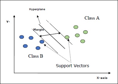
The main goal of SVMs is to divide the datasets into number of classes in order to find a maximum marginal hyperplane (MMH) which can be done in the following two steps −
Support Vector Machines will first generate hyperplanes iteratively that separates the classes in the best way.
After that it will choose the hyperplane that segregate the classes correctly.
Some important concepts in SVM are as follows −
Support Vectors − They may be defined as the datapoints which are closest to the hyperplane. Support vectors help in deciding the separating line.
Hyperplane − The decision plane or space that divides set of objects having different classes.
Margin − The gap between two lines on the closet data points of different classes is called margin.
Following diagrams will give you an insight about these SVM concepts −
SVM in Scikit-learn supports both sparse and dense sample vectors as input.
Classification of SVM
Scikit-learn provides three classes namely SVC, NuSVC and LinearSVC which can perform multiclass-class classification.
SVC
It is C-support vector classification whose implementation is based on libsvm. The module used by scikit-learn is sklearn.svm.SVC. This class handles the multiclass support according to one-vs-one scheme.
Parameters
Followings table consist the parameters used by sklearn.svm.SVC class −
| Sr.No | Parameter & Description |
|---|---|
| 1 |
C − float, optional, default = 1.0 It is the penalty parameter of the error term. |
| 2 |
kernel − string, optional, default = ‘rbf’ This parameter specifies the type of kernel to be used in the algorithm. we can choose any one among, ‘linear’, ‘poly’, ‘rbf’, ‘sigmoid’, ‘precomputed’. The default value of kernel would be ‘rbf’. |
| 3 |
degree − int, optional, default = 3 It represents the degree of the ‘poly’ kernel function and will be ignored by all other kernels. |
| 4 |
gamma − {‘scale’, ‘auto’} or float, It is the kernel coefficient for kernels ‘rbf’, ‘poly’ and ‘sigmoid’. |
| 5 |
optinal default − = ‘scale’ If you choose default i.e. gamma = ‘scale’ then the value of gamma to be used by SVC is 1/(𝑛_𝑓𝑒𝑎𝑡𝑢𝑟𝑒𝑠∗𝑋.𝑣𝑎𝑟()). On the other hand, if gamma= ‘auto’, it uses 1/𝑛_𝑓𝑒𝑎𝑡𝑢𝑟𝑒𝑠. |
| 6 |
coef0 − float, optional, Default=0.0 An independent term in kernel function which is only significant in ‘poly’ and ‘sigmoid’. |
| 7 |
tol − float, optional, default = 1.e-3 This parameter represents the stopping criterion for iterations. |
| 8 |
shrinking − Boolean, optional, default = True This parameter represents that whether we want to use shrinking heuristic or not. |
| 9 |
verbose − Boolean, default: false It enables or disable verbose output. Its default value is false. |
| 10 |
probability − boolean, optional, default = true This parameter enables or disables probability estimates. The default value is false, but it must be enabled before we call fit. |
| 11 |
max_iter − int, optional, default = -1 As name suggest, it represents the maximum number of iterations within the solver. Value -1 means there is no limit on the number of iterations. |
| 12 |
cache_size − float, optional This parameter will specify the size of the kernel cache. The value will be in MB(MegaBytes). |
| 13 |
random_state − int, RandomState instance or None, optional, default = none This parameter represents the seed of the pseudo random number generated which is used while shuffling the data. Followings are the options −
|
| 14 |
class_weight − {dict, ‘balanced’}, optional This parameter will set the parameter C of class j to 𝑐𝑙𝑎𝑠𝑠_𝑤𝑒𝑖𝑔ℎ𝑡[𝑗]∗𝐶 for SVC. If we use the default option, it means all the classes are supposed to have weight one. On the other hand, if you choose class_weight:balanced, it will use the values of y to automatically adjust weights. |
| 15 |
decision_function_shape − ovo’, ‘ovr’, default = ‘ovr’ This parameter will decide whether the algorithm will return ‘ovr’ (one-vs-rest) decision function of shape as all other classifiers, or the original ovo(one-vs-one) decision function of libsvm. |
| 16 |
break_ties − boolean, optional, default = false True − The predict will break ties according to the confidence values of decision_function False − The predict will return the first class among the tied classes. |
Attributes
Followings table consist the attributes used by sklearn.svm.SVC class −
| Sr.No | Attributes & Description |
|---|---|
| 1 |
support_ − array-like, shape = [n_SV] It returns the indices of support vectors. |
| 2 |
support_vectors_ − array-like, shape = [n_SV, n_features] It returns the support vectors. |
| 3 |
n_support_ − array-like, dtype=int32, shape = [n_class] It represents the number of support vectors for each class. |
| 4 |
dual_coef_ − array, shape = [n_class-1,n_SV] These are the coefficient of the support vectors in the decision function. |
| 5 |
coef_ − array, shape = [n_class * (n_class-1)/2, n_features] This attribute, only available in case of linear kernel, provides the weight assigned to the features. |
| 6 |
intercept_ − array, shape = [n_class * (n_class-1)/2] It represents the independent term (constant) in decision function. |
| 7 |
fit_status_ − int The output would be 0 if it is correctly fitted. The output would be 1 if it is incorrectly fitted. |
| 8 |
classes_ − array of shape = [n_classes] It gives the labels of the classes. |
Implementation Example
Like other classifiers, SVC also has to be fitted with following two arrays −
An array X holding the training samples. It is of size [n_samples, n_features].
An array Y holding the target values i.e. class labels for the training samples. It is of size [n_samples].
Following Python script uses sklearn.svm.SVC class −
import numpy as np
X = np.array([[-1, -1], [-2, -1], [1, 1], [2, 1]])
y = np.array([1, 1, 2, 2])
from sklearn.svm import SVC
SVCClf = SVC(kernel = 'linear',gamma = 'scale', shrinking = False,)
SVCClf.fit(X, y)
Output
SVC(C = 1.0, cache_size = 200, class_weight = None, coef0 = 0.0,
   decision_function_shape = 'ovr', degree = 3, gamma = 'scale', kernel = 'linear',
   max_iter = -1, probability = False, random_state = None, shrinking = False,
   tol = 0.001, verbose = False)
Example
Now, once fitted, we can get the weight vector with the help of following python script −
SVCClf.coef_
Output
array([[0.5, 0.5]])
Example
Similarly, we can get the value of other attributes as follows −
SVCClf.predict([[-0.5,-0.8]])
Output
array([1])
Example
SVCClf.n_support_
Output
array([1, 1])
Example
SVCClf.support_vectors_
Output
array(
   [
      [-1., -1.],
      [ 1., 1.]
   ]
)
Example
SVCClf.support_
Output
array([0, 2])
Example
SVCClf.intercept_
Output
array([-0.])
Example
SVCClf.fit_status_
Output
0
NuSVC
NuSVC is Nu Support Vector Classification. It is another class provided by scikit-learn which can perform multi-class classification. It is like SVC but NuSVC accepts slightly different sets of parameters. The parameter which is different from SVC is as follows −
nu − float, optional, default = 0.5
It represents an upper bound on the fraction of training errors and a lower bound of the fraction of support vectors. Its value should be in the interval of (o,1].
Rest of the parameters and attributes are same as of SVC.
Implementation Example
We can implement the same example using sklearn.svm.NuSVC class also.
import numpy as np
X = np.array([[-1, -1], [-2, -1], [1, 1], [2, 1]])
y = np.array([1, 1, 2, 2])
from sklearn.svm import NuSVC
NuSVCClf = NuSVC(kernel = 'linear',gamma = 'scale', shrinking = False,)
NuSVCClf.fit(X, y)
Output
NuSVC(cache_size = 200, class_weight = None, coef0 = 0.0,
   decision_function_shape = 'ovr', degree = 3, gamma = 'scale', kernel = 'linear',
   max_iter = -1, nu = 0.5, probability = False, random_state = None,
   shrinking = False, tol = 0.001, verbose = False)
We can get the outputs of rest of the attributes as did in the case of SVC.
LinearSVC
It is Linear Support Vector Classification. It is similar to SVC having kernel = ‘linear’. The difference between them is that LinearSVC implemented in terms of liblinear while SVC is implemented in libsvm. That’s the reason LinearSVC has more flexibility in the choice of penalties and loss functions. It also scales better to large number of samples.
If we talk about its parameters and attributes then it does not support ‘kernel’ because it is assumed to be linear and it also lacks some of the attributes like support_, support_vectors_, n_support_, fit_status_ and, dual_coef_.
However, it supports penalty and loss parameters as follows −
penalty − string, L1 or L2(default = ‘L2’)
This parameter is used to specify the norm (L1 or L2) used in penalization (regularization).
loss − string, hinge, squared_hinge (default = squared_hinge)
It represents the loss function where ‘hinge’ is the standard SVM loss and ‘squared_hinge’ is the square of hinge loss.
Implementation Example
Following Python script uses sklearn.svm.LinearSVC class −
from sklearn.svm import LinearSVC
from sklearn.datasets import make_classification
X, y = make_classification(n_features = 4, random_state = 0)
LSVCClf = LinearSVC(dual = False, random_state = 0, penalty = 'l1',tol = 1e-5)
LSVCClf.fit(X, y)
Output
LinearSVC(C = 1.0, class_weight = None, dual = False, fit_intercept = True,
   intercept_scaling = 1, loss = 'squared_hinge', max_iter = 1000,
   multi_class = 'ovr', penalty = 'l1', random_state = 0, tol = 1e-05, verbose = 0)
Example
Now, once fitted, the model can predict new values as follows −
LSVCClf.predict([[0,0,0,0]])
Output
[1]
Example
For the above example, we can get the weight vector with the help of following python script −
LSVCClf.coef_
Output
[[0. 0. 0.91214955 0.22630686]]
Example
Similarly, we can get the value of intercept with the help of following python script −
LSVCClf.intercept_
Output
[0.26860518]
Regression with SVM
As discussed earlier, SVM is used for both classification and regression problems. Scikit-learn’s method of Support Vector Classification (SVC) can be extended to solve regression problems as well. That extended method is called Support Vector Regression (SVR).
Basic similarity between SVM and SVR
The model created by SVC depends only on a subset of training data. Why? Because the cost function for building the model doesn’t care about training data points that lie outside the margin.
Whereas, the model produced by SVR (Support Vector Regression) also only depends on a subset of the training data. Why? Because the cost function for building the model ignores any training data points close to the model prediction.
Scikit-learn provides three classes namely SVR, NuSVR and LinearSVR as three different implementations of SVR.
SVR
It is Epsilon-support vector regression whose implementation is based on libsvm. As opposite to SVC There are two free parameters in the model namely ‘C’ and ‘epsilon’.
epsilon − float, optional, default = 0.1
It represents the epsilon in the epsilon-SVR model, and specifies the epsilon-tube within which no penalty is associated in the training loss function with points predicted within a distance epsilon from the actual value.
Rest of the parameters and attributes are similar as we used in SVC.
Implementation Example
Following Python script uses sklearn.svm.SVR class −
from sklearn import svm
X = [[1, 1], [2, 2]]
y = [1, 2]
SVRReg = svm.SVR(kernel = ’linear’, gamma = ’auto’)
SVRReg.fit(X, y)
Output
SVR(C = 1.0, cache_size = 200, coef0 = 0.0, degree = 3, epsilon = 0.1, gamma = 'auto',
   kernel = 'linear', max_iter = -1, shrinking = True, tol = 0.001, verbose = False)
Example
Now, once fitted, we can get the weight vector with the help of following python script −
SVRReg.coef_
Output
array([[0.4, 0.4]])
Example
Similarly, we can get the value of other attributes as follows −
SVRReg.predict([[1,1]])
Output
array([1.1])
Similarly, we can get the values of other attributes as well.
NuSVR
NuSVR is Nu Support Vector Regression. It is like NuSVC, but NuSVR uses a parameter nu to control the number of support vectors. And moreover, unlike NuSVC where nu replaced C parameter, here it replaces epsilon.
Implementation Example
Following Python script uses sklearn.svm.SVR class −
from sklearn.svm import NuSVR
import numpy as np
n_samples, n_features = 20, 15
np.random.seed(0)
y = np.random.randn(n_samples)
X = np.random.randn(n_samples, n_features)
NuSVRReg = NuSVR(kernel = 'linear', gamma = 'auto',C = 1.0, nu = 0.1)^M
NuSVRReg.fit(X, y)
Output
NuSVR(C = 1.0, cache_size = 200, coef0 = 0.0, degree = 3, gamma = 'auto',
   kernel = 'linear', max_iter = -1, nu = 0.1, shrinking = True, tol = 0.001,
   verbose = False)
Example
Now, once fitted, we can get the weight vector with the help of following python script −
NuSVRReg.coef_
Output
array(
   [
      [-0.14904483, 0.04596145, 0.22605216, -0.08125403, 0.06564533,
      0.01104285, 0.04068767, 0.2918337 , -0.13473211, 0.36006765,
      -0.2185713 , -0.31836476, -0.03048429, 0.16102126, -0.29317051]
   ]
)
Similarly, we can get the value of other attributes as well.
LinearSVR
It is Linear Support Vector Regression. It is similar to SVR having kernel = ‘linear’. The difference between them is that LinearSVR implemented in terms of liblinear, while SVC implemented in libsvm. That’s the reason LinearSVR has more flexibility in the choice of penalties and loss functions. It also scales better to large number of samples.
If we talk about its parameters and attributes then it does not support ‘kernel’ because it is assumed to be linear and it also lacks some of the attributes like support_, support_vectors_, n_support_, fit_status_ and, dual_coef_.
However, it supports ‘loss’ parameters as follows −
loss − string, optional, default = ‘epsilon_insensitive’
It represents the loss function where epsilon_insensitive loss is the L1 loss and the squared epsilon-insensitive loss is the L2 loss.
Implementation Example
Following Python script uses sklearn.svm.LinearSVR class −
from sklearn.svm import LinearSVR
from sklearn.datasets import make_regression
X, y = make_regression(n_features = 4, random_state = 0)
LSVRReg = LinearSVR(dual = False, random_state = 0,
loss = 'squared_epsilon_insensitive',tol = 1e-5)
LSVRReg.fit(X, y)
Output
LinearSVR(
   C=1.0, dual=False, epsilon=0.0, fit_intercept=True,
   intercept_scaling=1.0, loss='squared_epsilon_insensitive',
   max_iter=1000, random_state=0, tol=1e-05, verbose=0
)
Example
Now, once fitted, the model can predict new values as follows −
LSRReg.predict([[0,0,0,0]])
Output
array([-0.01041416])
Example
For the above example, we can get the weight vector with the help of following python script −
LSRReg.coef_
Output
array([20.47354746, 34.08619401, 67.23189022, 87.47017787])
Example
Similarly, we can get the value of intercept with the help of following python script −
LSRReg.intercept_
Output
array([-0.01041416])
Scikit Learn - Anomaly Detection
Here, we will learn about what is anomaly detection in Sklearn and how it is used in identification of the data points.
Anomaly detection is a technique used to identify data points in dataset that does not fit well with the rest of the data. It has many applications in business such as fraud detection, intrusion detection, system health monitoring, surveillance, and predictive maintenance. Anomalies, which are also called outlier, can be divided into following three categories −
Point anomalies − It occurs when an individual data instance is considered as anomalous w.r.t the rest of the data.
Contextual anomalies − Such kind of anomaly is context specific. It occurs if a data instance is anomalous in a specific context.
Collective anomalies − It occurs when a collection of related data instances is anomalous w.r.t entire dataset rather than individual values.
Methods
Two methods namely outlier detection and novelty detection can be used for anomaly detection. It’s necessary to see the distinction between them.
Outlier detection
The training data contains outliers that are far from the rest of the data. Such outliers are defined as observations. That’s the reason, outlier detection estimators always try to fit the region having most concentrated training data while ignoring the deviant observations. It is also known as unsupervised anomaly detection.
Novelty detection
It is concerned with detecting an unobserved pattern in new observations which is not included in training data. Here, the training data is not polluted by the outliers. It is also known as semi-supervised anomaly detection.
There are set of ML tools, provided by scikit-learn, which can be used for both outlier detection as well novelty detection. These tools first implementing object learning from the data in an unsupervised by using fit () method as follows −
estimator.fit(X_train)
Now, the new observations would be sorted as inliers (labeled 1) or outliers (labeled -1) by using predict() method as follows −
estimator.fit(X_test)
The estimator will first compute the raw scoring function and then predict method will make use of threshold on that raw scoring function. We can access this raw scoring function with the help of score_sample method and can control the threshold by contamination parameter.
We can also define decision_function method that defines outliers as negative value and inliers as non-negative value.
estimator.decision_function(X_test)
Sklearn algorithms for Outlier Detection
Let us begin by understanding what an elliptic envelop is.
Fitting an elliptic envelop
This algorithm assume that regular data comes from a known distribution such as Gaussian distribution. For outlier detection, Scikit-learn provides an object named covariance.EllipticEnvelop.
This object fits a robust covariance estimate to the data, and thus, fits an ellipse to the central data points. It ignores the points outside the central mode.
Parameters
Following table consist the parameters used by sklearn. covariance.EllipticEnvelop method −
| Sr.No | Parameter & Description |
|---|---|
| 1 |
store_precision − Boolean, optional, default = True We can specify it if the estimated precision is stored. |
| 2 |
assume_centered − Boolean, optional, default = False If we set it False, it will compute the robust location and covariance directly with the help of FastMCD algorithm. On the other hand, if set True, it will compute the support of robust location and covarian. |
| 3 |
support_fraction − float in (0., 1.), optional, default = None This parameter tells the method that how much proportion of points to be included in the support of the raw MCD estimates. |
| 4 |
contamination − float in (0., 1.), optional, default = 0.1 It provides the proportion of the outliers in the data set. |
| 5 |
random_state − int, RandomState instance or None, optional, default = none This parameter represents the seed of the pseudo random number generated which is used while shuffling the data. Followings are the options −
|
Attributes
Following table consist the attributes used by sklearn. covariance.EllipticEnvelop method −
| Sr.No | Attributes & Description |
|---|---|
| 1 |
support_ − array-like, shape(n_samples,) It represents the mask of the observations used to compute robust estimates of location and shape. |
| 2 |
location_ − array-like, shape (n_features) It returns the estimated robust location. |
| 3 |
covariance_ − array-like, shape (n_features, n_features) It returns the estimated robust covariance matrix. |
| 4 |
precision_ − array-like, shape (n_features, n_features) It returns the estimated pseudo inverse matrix. |
| 5 |
offset_ − float It is used to define the decision function from the raw scores. decision_function = score_samples -offset_ |
Implementation Example
import numpy as np^M
from sklearn.covariance import EllipticEnvelope^M
true_cov = np.array([[.5, .6],[.6, .4]])
X = np.random.RandomState(0).multivariate_normal(mean = [0, 0], cov=true_cov,size=500)
cov = EllipticEnvelope(random_state = 0).fit(X)^M
# Now we can use predict method. It will return 1 for an inlier and -1 for an outlier.
cov.predict([[0, 0],[2, 2]])
Output
array([ 1, -1])
Isolation Forest
In case of high-dimensional dataset, one efficient way for outlier detection is to use random forests. The scikit-learn provides ensemble.IsolationForest method that isolates the observations by randomly selecting a feature. Afterwards, it randomly selects a value between the maximum and minimum values of the selected features.
Here, the number of splitting needed to isolate a sample is equivalent to path length from the root node to the terminating node.
Parameters
Followings table consist the parameters used by sklearn. ensemble.IsolationForest method −
| Sr.No | Parameter & Description |
|---|---|
| 1 |
n_estimators − int, optional, default = 100 It represents the number of base estimators in the ensemble. |
| 2 |
max_samples − int or float, optional, default = “auto” It represents the number of samples to be drawn from X to train each base estimator. If we choose int as its value, it will draw max_samples samples. If we choose float as its value, it will draw max_samples ∗ 𝑋.shape[0] samples. And, if we choose auto as its value, it will draw max_samples = min(256,n_samples). |
| 3 |
support_fraction − float in (0., 1.), optional, default = None This parameter tells the method that how much proportion of points to be included in the support of the raw MCD estimates. |
| 4 |
contamination − auto or float, optional, default = auto It provides the proportion of the outliers in the data set. If we set it default i.e. auto, it will determine the threshold as in the original paper. If set to float, the range of contamination will be in the range of [0,0.5]. |
| 5 |
random_state − int, RandomState instance or None, optional, default = none This parameter represents the seed of the pseudo random number generated which is used while shuffling the data. Followings are the options −
|
| 6 |
max_features − int or float, optional (default = 1.0) It represents the number of features to be drawn from X to train each base estimator. If we choose int as its value, it will draw max_features features. If we choose float as its value, it will draw max_features * X.shape[𝟏] samples. |
| 7 | bootstrap − Boolean, optional (default = False) Its default option is False which means the sampling would be performed without replacement. And on the other hand, if set to True, means individual trees are fit on a random subset of the training data sampled with replacement. |
| 8 |
n_jobs − int or None, optional (default = None) It represents the number of jobs to be run in parallel for fit() and predict() methods both. |
| 9 |
verbose − int, optional (default = 0) This parameter controls the verbosity of the tree building process. |
| 10 |
warm_start − Bool, optional (default=False) If warm_start = true, we can reuse previous calls solution to fit and can add more estimators to the ensemble. But if is set to false, we need to fit a whole new forest. |
Attributes
Following table consist the attributes used by sklearn. ensemble.IsolationForest method −
| Sr.No | Attributes & Description |
|---|---|
| 1 |
estimators_ − list of DecisionTreeClassifier Providing the collection of all fitted sub-estimators. |
| 2 |
max_samples_ − integer It provides the actual number of samples used. |
| 3 |
offset_ − float It is used to define the decision function from the raw scores. decision_function = score_samples -offset_ |
Implementation Example
The Python script below will use sklearn. ensemble.IsolationForest method to fit 10 trees on given data
from sklearn.ensemble import IsolationForest
import numpy as np
X = np.array([[-1, -2], [-3, -3], [-3, -4], [0, 0], [-50, 60]])
OUTDClf = IsolationForest(n_estimators = 10)
OUTDclf.fit(X)
Output
IsolationForest(
   behaviour = 'old', bootstrap = False, contamination='legacy',
   max_features = 1.0, max_samples = 'auto', n_estimators = 10, n_jobs=None,
   random_state = None, verbose = 0
)
Local Outlier Factor
Local Outlier Factor (LOF) algorithm is another efficient algorithm to perform outlier detection on high dimension data. The scikit-learn provides neighbors.LocalOutlierFactor method that computes a score, called local outlier factor, reflecting the degree of anomality of the observations. The main logic of this algorithm is to detect the samples that have a substantially lower density than its neighbors. Thats why it measures the local density deviation of given data points w.r.t. their neighbors.
Parameters
Followings table consist the parameters used by sklearn. neighbors.LocalOutlierFactor method
| Sr.No | Parameter & Description |
|---|---|
| 1 |
n_neighbors − int, optional, default = 20 It represents the number of neighbors use by default for kneighbors query. All samples would be used if . |
| 2 |
algorithm − optional Which algorithm to be used for computing nearest neighbors.
|
| 3 |
leaf_size − int, optional, default = 30 The value of this parameter can affect the speed of the construction and query. It also affects the memory required to store the tree. This parameter is passed to BallTree or KdTree algorithms. |
| 4 |
contamination − auto or float, optional, default = auto It provides the proportion of the outliers in the data set. If we set it default i.e. auto, it will determine the threshold as in the original paper. If set to float, the range of contamination will be in the range of [0,0.5]. |
| 5 |
metric − string or callable, default It represents the metric used for distance computation. |
| 6 |
P − int, optional (default = 2) It is the parameter for the Minkowski metric. P=1 is equivalent to using manhattan_distance i.e. L1, whereas P=2 is equivalent to using euclidean_distance i.e. L2. |
| 7 |
novelty − Boolean, (default = False) By default, LOF algorithm is used for outlier detection but it can be used for novelty detection if we set novelty = true. |
| 8 |
n_jobs − int or None, optional (default = None) It represents the number of jobs to be run in parallel for fit() and predict() methods both. |
Attributes
Following table consist the attributes used by sklearn.neighbors.LocalOutlierFactor method −
| Sr.No | Attributes & Description |
|---|---|
| 1 |
negative_outlier_factor_ − numpy array, shape(n_samples,) Providing opposite LOF of the training samples. |
| 2 |
n_neighbors_ − integer It provides the actual number of neighbors used for neighbors queries. |
| 3 |
offset_ − float It is used to define the binary labels from the raw scores. |
Implementation Example
The Python script given below will use sklearn.neighbors.LocalOutlierFactor method to construct NeighborsClassifier class from any array corresponding our data set
from sklearn.neighbors import NearestNeighbors
samples = [[0., 0., 0.], [0., .5, 0.], [1., 1., .5]]
LOFneigh = NearestNeighbors(n_neighbors = 1, algorithm = "ball_tree",p=1)
LOFneigh.fit(samples)
Output
NearestNeighbors(
   algorithm = 'ball_tree', leaf_size = 30, metric='minkowski',
   metric_params = None, n_jobs = None, n_neighbors = 1, p = 1, radius = 1.0
)
Example
Now, we can ask from this constructed classifier is the closet point to [0.5, 1., 1.5] by using the following python script −
print(neigh.kneighbors([[.5, 1., 1.5]])
Output
(array([[1.7]]), array([[1]], dtype = int64))
One-Class SVM
The One-Class SVM, introduced by Schölkopf et al., is the unsupervised Outlier Detection. It is also very efficient in high-dimensional data and estimates the support of a high-dimensional distribution. It is implemented in the Support Vector Machines module in the Sklearn.svm.OneClassSVM object. For defining a frontier, it requires a kernel (mostly used is RBF) and a scalar parameter.
For better understanding let's fit our data with svm.OneClassSVM object −
Example
from sklearn.svm import OneClassSVM
X = [[0], [0.89], [0.90], [0.91], [1]]
OSVMclf = OneClassSVM(gamma = 'scale').fit(X)
Now, we can get the score_samples for input data as follows −
OSVMclf.score_samples(X)
Output
array([1.12218594, 1.58645126, 1.58673086, 1.58645127, 1.55713767])
Scikit Learn - K-Nearest Neighbors (KNN)
This chapter will help you in understanding the nearest neighbor methods in Sklearn.
Neighbor based learning method are of both types namely supervised and unsupervised. Supervised neighbors-based learning can be used for both classification as well as regression predictive problems but, it is mainly used for classification predictive problems in industry.
Neighbors based learning methods do not have a specialised training phase and uses all the data for training while classification. It also does not assume anything about the underlying data. That’s the reason they are lazy and non-parametric in nature.
The main principle behind nearest neighbor methods is −
To find a predefined number of training samples closet in distance to the new data point
Predict the label from these number of training samples.
Here, the number of samples can be a user-defined constant like in K-nearest neighbor learning or vary based on the local density of point like in radius-based neighbor learning.
sklearn.neighbors Module
Scikit-learn have sklearn.neighbors module that provides functionality for both unsupervised and supervised neighbors-based learning methods. As input, the classes in this module can handle either NumPy arrays or scipy.sparse matrices.
Types of algorithms
Different types of algorithms which can be used in neighbor-based methods’ implementation are as follows −
Brute Force
The brute-force computation of distances between all pairs of points in the dataset provides the most naïve neighbor search implementation. Mathematically, for N samples in D dimensions, brute-force approach scales as 0[DN2]
For small data samples, this algorithm can be very useful, but it becomes infeasible as and when number of samples grows. Brute force neighbor search can be enabled by writing the keyword algorithm=’brute’.
K-D Tree
One of the tree-based data structures that have been invented to address the computational inefficiencies of the brute-force approach, is KD tree data structure. Basically, the KD tree is a binary tree structure which is called K-dimensional tree. It recursively partitions the parameters space along the data axes by dividing it into nested orthographic regions into which the data points are filled.
Advantages
Following are some advantages of K-D tree algorithm −
Construction is fast − As the partitioning is performed only along the data axes, K-D tree’s construction is very fast.
Less distance computations − This algorithm takes very less distance computations to determine the nearest neighbor of a query point. It only takes 𝑶[𝐥𝐨𝐠 (𝑵)] distance computations.
Disadvantages
Fast for only low-dimensional neighbor searches − It is very fast for low-dimensional (D < 20) neighbor searches but as and when D grow it becomes inefficient. As the partitioning is performed only along the data axes,
K-D tree neighbor searches can be enabled by writing the keyword algorithm=’kd_tree’.
Ball Tree
As we know that KD Tree is inefficient in higher dimensions, hence, to address this inefficiency of KD Tree, Ball tree data structure was developed. Mathematically, it recursively divides the data, into nodes defined by a centroid C and radius r, in such a way that each point in the node lies within the hyper-sphere defined by centroid C and radius r. It uses triangle inequality, given below, which reduces the number of candidate points for a neighbor search
$$\arrowvert X+Y\arrowvert\leq \arrowvert X\arrowvert+\arrowvert Y\arrowvert$$Advantages
Following are some advantages of Ball Tree algorithm −
Efficient on highly structured data − As ball tree partition the data in a series of nesting hyper-spheres, it is efficient on highly structured data.
Out-performs KD-tree − Ball tree out-performs KD tree in high dimensions because it has spherical geometry of the ball tree nodes.
Disadvantages
Costly − Partition the data in a series of nesting hyper-spheres makes its construction very costly.
Ball tree neighbor searches can be enabled by writing the keyword algorithm=’ball_tree’.
Choosing Nearest Neighbors Algorithm
The choice of an optimal algorithm for a given dataset depends upon the following factors −
Number of samples (N) and Dimensionality (D)
These are the most important factors to be considered while choosing Nearest Neighbor algorithm. It is because of the reasons given below −
The query time of Brute Force algorithm grows as O[DN].
The query time of Ball tree algorithm grows as O[D log(N)].
The query time of KD tree algorithm changes with D in a strange manner that is very difficult to characterize. When D < 20, the cost is O[D log(N)] and this algorithm is very efficient. On the other hand, it is inefficient in case when D > 20 because the cost increases to nearly O[DN].
Data Structure
Another factor that affect the performance of these algorithms is intrinsic dimensionality of the data or sparsity of the data. It is because the query times of Ball tree and KD tree algorithms can be greatly influenced by it. Whereas, the query time of Brute Force algorithm is unchanged by data structure. Generally, Ball tree and KD tree algorithms produces faster query time when implanted on sparser data with smaller intrinsic dimensionality.
Number of Neighbors (k)
The number of neighbors (k) requested for a query point affects the query time of Ball tree and KD tree algorithms. Their query time becomes slower as number of neighbors (k) increases. Whereas the query time of Brute Force will remain unaffected by the value of k.
Number of query points
Because, they need construction phase, both KD tree and Ball tree algorithms will be effective if there are large number of query points. On the other hand, if there are a smaller number of query points, Brute Force algorithm performs better than KD tree and Ball tree algorithms.
Scikit Learn - KNN Learning
k-NN (k-Nearest Neighbor), one of the simplest machine learning algorithms, is non-parametric and lazy in nature. Non-parametric means that there is no assumption for the underlying data distribution i.e. the model structure is determined from the dataset. Lazy or instance-based learning means that for the purpose of model generation, it does not require any training data points and whole training data is used in the testing phase.
The k-NN algorithm consist of the following two steps −
Step 1
In this step, it computes and stores the k nearest neighbors for each sample in the training set.
Step 2
In this step, for an unlabeled sample, it retrieves the k nearest neighbors from dataset. Then among these k-nearest neighbors, it predicts the class through voting (class with majority votes wins).
The module, sklearn.neighbors that implements the k-nearest neighbors algorithm, provides the functionality for unsupervised as well as supervised neighbors-based learning methods.
The unsupervised nearest neighbors implement different algorithms (BallTree, KDTree or Brute Force) to find the nearest neighbor(s) for each sample. This unsupervised version is basically only step 1, which is discussed above, and the foundation of many algorithms (KNN and K-means being the famous one) which require the neighbor search. In simple words, it is Unsupervised learner for implementing neighbor searches.
On the other hand, the supervised neighbors-based learning is used for classification as well as regression.
Unsupervised KNN Learning
As discussed, there exist many algorithms like KNN and K-Means that requires nearest neighbor searches. That is why Scikit-learn decided to implement the neighbor search part as its own “learner”. The reason behind making neighbor search as a separate learner is that computing all pairwise distance for finding a nearest neighbor is obviously not very efficient. Let’s see the module used by Sklearn to implement unsupervised nearest neighbor learning along with example.
Scikit-learn module
sklearn.neighbors.NearestNeighbors is the module used to implement unsupervised nearest neighbor learning. It uses specific nearest neighbor algorithms named BallTree, KDTree or Brute Force. In other words, it acts as a uniform interface to these three algorithms.
Parameters
Followings table consist the parameters used by NearestNeighbors module −
| Sr.No | Parameter & Description |
|---|---|
| 1 |
n_neighbors − int, optional The number of neighbors to get. The default value is 5. |
| 2 |
radius − float, optional It limits the distance of neighbors to returns. The default value is 1.0. |
| 3 |
algorithm − {‘auto’, ‘ball_tree’, ‘kd_tree’, ‘brute’}, optional This parameter will take the algorithm (BallTree, KDTree or Brute-force) you want to use to compute the nearest neighbors. If you will provide ‘auto’, it will attempt to decide the most appropriate algorithm based on the values passed to fit method. |
| 4 |
leaf_size − int, optional It can affect the speed of the construction & query as well as the memory required to store the tree. It is passed to BallTree or KDTree. Although the optimal value depends on the nature of the problem, its default value is 30. |
| 5 |
metric − string or callable It is the metric to use for distance computation between points. We can pass it as a string or callable function. In case of callable function, the metric is called on each pair of rows and the resulting value is recorded. It is less efficient than passing the metric name as a string. We can choose from metric from scikit-learn or scipy.spatial.distance. the valid values are as follows − Scikit-learn − [‘cosine’,’manhattan’,‘Euclidean’, ‘l1’,’l2’, ‘cityblock’] Scipy.spatial.distance − [‘braycurtis’,‘canberra’,‘chebyshev’,‘dice’,‘hamming’,‘jaccard’, ‘correlation’,‘kulsinski’,‘mahalanobis’,‘minkowski’,‘rogerstanimoto’,‘russellrao’, ‘sokalmicheme’,’sokalsneath’, ‘seuclidean’, ‘sqeuclidean’, ‘yule’]. The default metric is ‘Minkowski’. |
| 6 |
P − integer, optional It is the parameter for the Minkowski metric. The default value is 2 which is equivalent to using Euclidean_distance(l2). |
| 7 |
metric_params − dict, optional This is the additional keyword arguments for the metric function. The default value is None. |
| 8 |
N_jobs − int or None, optional It reprsetst the numer of parallel jobs to run for neighbor search. The default value is None. |
Implementation Example
The example below will find the nearest neighbors between two sets of data by using the sklearn.neighbors.NearestNeighbors module.
First, we need to import the required module and packages −
from sklearn.neighbors import NearestNeighbors
import numpy as np
Now, after importing the packages, define the sets of data in between we want to find the nearest neighbors −
Input_data = np.array([[-1, 1], [-2, 2], [-3, 3], [1, 2], [2, 3], [3, 4],[4, 5]])
Next, apply the unsupervised learning algorithm, as follows −
nrst_neigh = NearestNeighbors(n_neighbors = 3, algorithm = 'ball_tree')
Next, fit the model with input data set.
nrst_neigh.fit(Input_data)
Now, find the K-neighbors of data set. It will return the indices and distances of the neighbors of each point.
distances, indices = nbrs.kneighbors(Input_data)
indices
Output
array(
   [
      [0, 1, 3],
      [1, 2, 0],
      [2, 1, 0],
      [3, 4, 0],
      [4, 5, 3],
      [5, 6, 4],
      [6, 5, 4]
   ], dtype = int64
)
distances
Output
array(
   [
      [0. , 1.41421356, 2.23606798],
      [0. , 1.41421356, 1.41421356],
      [0. , 1.41421356, 2.82842712],
      [0. , 1.41421356, 2.23606798],
      [0. , 1.41421356, 1.41421356],
      [0. , 1.41421356, 1.41421356],
      [0. , 1.41421356, 2.82842712]
   ]
)
The above output shows that the nearest neighbor of each point is the point itself i.e. at zero. It is because the query set matches the training set.
Example
We can also show a connection between neighboring points by producing a sparse graph as follows −
nrst_neigh.kneighbors_graph(Input_data).toarray()
Output
array(
   [
      [1., 1., 0., 1., 0., 0., 0.],
      [1., 1., 1., 0., 0., 0., 0.],
      [1., 1., 1., 0., 0., 0., 0.],
      [1., 0., 0., 1., 1., 0., 0.],
      [0., 0., 0., 1., 1., 1., 0.],
      [0., 0., 0., 0., 1., 1., 1.],
      [0., 0., 0., 0., 1., 1., 1.]
   ]
)
Once we fit the unsupervised NearestNeighbors model, the data will be stored in a data structure based on the value set for the argument ‘algorithm’. After that we can use this unsupervised learner’s kneighbors in a model which requires neighbor searches.
Complete working/executable program
from sklearn.neighbors import NearestNeighbors
import numpy as np
Input_data = np.array([[-1, 1], [-2, 2], [-3, 3], [1, 2], [2, 3], [3, 4],[4, 5]])
nrst_neigh = NearestNeighbors(n_neighbors = 3, algorithm='ball_tree')
nrst_neigh.fit(Input_data)
distances, indices = nbrs.kneighbors(Input_data)
indices
distances
nrst_neigh.kneighbors_graph(Input_data).toarray()
Supervised KNN Learning
The supervised neighbors-based learning is used for following −
- Classification, for the data with discrete labels
- Regression, for the data with continuous labels.
Nearest Neighbor Classifier
We can understand Neighbors-based classification with the help of following two characteristics −
- It is computed from a simple majority vote of the nearest neighbors of each point.
- It simply stores instances of the training data, that’s why it is a type of non-generalizing learning.
Scikit-learn modules
Followings are the two different types of nearest neighbor classifiers used by scikit-learn −
| S.No. | Classifiers & Description | 1. | KNeighborsClassifier
The K in the name of this classifier represents the k nearest neighbors, where k is an integer value specified by the user. Hence as the name suggests, this classifier implements learning based on the k nearest neighbors. The choice of the value of k is dependent on data. |
|---|---|
| 2. | RadiusNeighborsClassifier
The Radius in the name of this classifier represents the nearest neighbors within a specified radius r, where r is a floating-point value specified by the user. Hence as the name suggests, this classifier implements learning based on the number neighbors within a fixed radius r of each training point. |
Nearest Neighbor Regressor
It is used in the cases where data labels are continuous in nature. The assigned data labels are computed on the basis on the mean of the labels of its nearest neighbors.
Followings are the two different types of nearest neighbor regressors used by scikit-learn −
KNeighborsRegressor
The K in the name of this regressor represents the k nearest neighbors, where k is an integer value specified by the user. Hence, as the name suggests, this regressor implements learning based on the k nearest neighbors. The choice of the value of k is dependent on data. Let’s understand it more with the help of an implementation example.
Followings are the two different types of nearest neighbor regressors used by scikit-learn −
Implementation Example
In this example, we will be implementing KNN on data set named Iris Flower data set by using scikit-learn KNeighborsRegressor.
First, import the iris dataset as follows −
from sklearn.datasets import load_iris
iris = load_iris()
Now, we need to split the data into training and testing data. We will be using Sklearn train_test_split function to split the data into the ratio of 70 (training data) and 20 (testing data) −
X = iris.data[:, :4]
y = iris.target
from sklearn.model_selection import train_test_split
X_train, X_test, y_train, y_test = train_test_split(X, y, test_size = 0.20)
Next, we will be doing data scaling with the help of Sklearn preprocessing module as follows −
from sklearn.preprocessing import StandardScaler
scaler = StandardScaler()
scaler.fit(X_train)
X_train = scaler.transform(X_train)
X_test = scaler.transform(X_test)
Next, import the KNeighborsRegressor class from Sklearn and provide the value of neighbors as follows.
Example
import numpy as np
from sklearn.neighbors import KNeighborsRegressor
knnr = KNeighborsRegressor(n_neighbors = 8)
knnr.fit(X_train, y_train)
Output
KNeighborsRegressor(
   algorithm = 'auto', leaf_size = 30, metric = 'minkowski',
   metric_params = None, n_jobs = None, n_neighbors = 8, p = 2,
   weights = 'uniform'
)
Example
Now, we can find the MSE (Mean Squared Error) as follows −
print ("The MSE is:",format(np.power(y-knnr.predict(X),4).mean()))
Output
The MSE is: 4.4333349609375
Example
Now, use it to predict the value as follows −
X = [[0], [1], [2], [3]]
y = [0, 0, 1, 1]
from sklearn.neighbors import KNeighborsRegressor
knnr = KNeighborsRegressor(n_neighbors = 3)
knnr.fit(X, y)
print(knnr.predict([[2.5]]))
Output
[0.66666667]
Complete working/executable program
from sklearn.datasets import load_iris
iris = load_iris()
X = iris.data[:, :4]
y = iris.target
from sklearn.model_selection import train_test_split
X_train, X_test, y_train, y_test = train_test_split(X, y, test_size=0.20)
from sklearn.preprocessing import StandardScaler
scaler = StandardScaler()

scaler.fit(X_train)
X_train = scaler.transform(X_train)
X_test = scaler.transform(X_test)

import numpy as np
from sklearn.neighbors import KNeighborsRegressor
knnr = KNeighborsRegressor(n_neighbors=8)
knnr.fit(X_train, y_train)

print ("The MSE is:",format(np.power(y-knnr.predict(X),4).mean()))

X = [[0], [1], [2], [3]]
y = [0, 0, 1, 1]
from sklearn.neighbors import KNeighborsRegressor
knnr = KNeighborsRegressor(n_neighbors=3)
knnr.fit(X, y)
print(knnr.predict([[2.5]]))
RadiusNeighborsRegressor
The Radius in the name of this regressor represents the nearest neighbors within a specified radius r, where r is a floating-point value specified by the user. Hence as the name suggests, this regressor implements learning based on the number neighbors within a fixed radius r of each training point. Let’s understand it more with the help if an implementation example −
Implementation Example
In this example, we will be implementing KNN on data set named Iris Flower data set by using scikit-learn RadiusNeighborsRegressor −
First, import the iris dataset as follows −
from sklearn.datasets import load_iris
iris = load_iris()
Now, we need to split the data into training and testing data. We will be using Sklearn train_test_split function to split the data into the ratio of 70 (training data) and 20 (testing data) −
X = iris.data[:, :4]
y = iris.target
from sklearn.model_selection import train_test_split
X_train, X_test, y_train, y_test = train_test_split(X, y, test_size=0.20)
Next, we will be doing data scaling with the help of Sklearn preprocessing module as follows −
from sklearn.preprocessing import StandardScaler
scaler = StandardScaler()
scaler.fit(X_train)
X_train = scaler.transform(X_train)
X_test = scaler.transform(X_test)
Next, import the RadiusneighborsRegressor class from Sklearn and provide the value of radius as follows −
import numpy as np
from sklearn.neighbors import RadiusNeighborsRegressor
knnr_r = RadiusNeighborsRegressor(radius=1)
knnr_r.fit(X_train, y_train)
Example
Now, we can find the MSE (Mean Squared Error) as follows −
print ("The MSE is:",format(np.power(y-knnr_r.predict(X),4).mean()))
Output
The MSE is: The MSE is: 5.666666666666667
Example
Now, use it to predict the value as follows −
X = [[0], [1], [2], [3]]
y = [0, 0, 1, 1]
from sklearn.neighbors import RadiusNeighborsRegressor
knnr_r = RadiusNeighborsRegressor(radius=1)
knnr_r.fit(X, y)
print(knnr_r.predict([[2.5]]))
Output
[1.]
Complete working/executable program
from sklearn.datasets import load_iris

iris = load_iris()

X = iris.data[:, :4]
y = iris.target
from sklearn.model_selection import train_test_split
X_train, X_test, y_train, y_test = train_test_split(X, y, test_size = 0.20)
from sklearn.preprocessing import StandardScaler
scaler = StandardScaler()
scaler.fit(X_train)
X_train = scaler.transform(X_train)
X_test = scaler.transform(X_test)
import numpy as np
from sklearn.neighbors import RadiusNeighborsRegressor
knnr_r = RadiusNeighborsRegressor(radius = 1)
knnr_r.fit(X_train, y_train)
print ("The MSE is:",format(np.power(y-knnr_r.predict(X),4).mean()))
X = [[0], [1], [2], [3]]
y = [0, 0, 1, 1]
from sklearn.neighbors import RadiusNeighborsRegressor
knnr_r = RadiusNeighborsRegressor(radius = 1)
knnr_r.fit(X, y)
print(knnr_r.predict([[2.5]]))
Scikit Learn - Classification with Naïve Bayes
Naïve Bayes methods are a set of supervised learning algorithms based on applying Bayes’ theorem with a strong assumption that all the predictors are independent to each other i.e. the presence of a feature in a class is independent to the presence of any other feature in the same class. This is naïve assumption that is why these methods are called Naïve Bayes methods.
Bayes theorem states the following relationship in order to find the posterior probability of class i.e. the probability of a label and some observed features, $P\left(\begin{array}{c} Y\arrowvert features\end{array}\right)$.
$$P\left(\begin{array}{c} Y\arrowvert features\end{array}\right)=\left(\frac{P\lgroup Y\rgroup P\left(\begin{array}{c} features\arrowvert Y\end{array}\right)}{P\left(\begin{array}{c} features\end{array}\right)}\right)$$Here, $P\left(\begin{array}{c} Y\arrowvert features\end{array}\right)$ is the posterior probability of class.
$P\left(\begin{array}{c} Y\end{array}\right)$ is the prior probability of class.
$P\left(\begin{array}{c} features\arrowvert Y\end{array}\right)$ is the likelihood which is the probability of predictor given class.
$P\left(\begin{array}{c} features\end{array}\right)$ is the prior probability of predictor.
The Scikit-learn provides different naïve Bayes classifiers models namely Gaussian, Multinomial, Complement and Bernoulli. All of them differ mainly by the assumption they make regarding the distribution of 𝑷$P\left(\begin{array}{c} features\arrowvert Y\end{array}\right)$ i.e. the probability of predictor given class.
| Sr.No | Model & Description |
|---|---|
| 1 |
Gaussian Naïve Bayes
Gaussian Naïve Bayes classifier assumes that the data from each label is drawn from a simple Gaussian distribution. |
| 2 |
Multinomial Naïve Bayes
It assumes that the features are drawn from a simple Multinomial distribution. |
| 3 |
Bernoulli Naïve Bayes
The assumption in this model is that the features binary (0s and 1s) in nature. An application of Bernoulli Naïve Bayes classification is Text classification with ‘bag of words’ model |
| 4 |
Complement Naïve Bayes
It was designed to correct the severe assumptions made by Multinomial Bayes classifier. This kind of NB classifier is suitable for imbalanced data sets |
Building Naïve Bayes Classifier
We can also apply Naïve Bayes classifier on Scikit-learn dataset. In the example below, we are applying GaussianNB and fitting the breast_cancer dataset of Scikit-leran.
Example
Import Sklearn
from sklearn.datasets import load_breast_cancer
from sklearn.model_selection import train_test_split
data = load_breast_cancer()
label_names = data['target_names']
labels = data['target']
feature_names = data['feature_names']
features = data['data']
   print(label_names)
   print(labels[0])
   print(feature_names[0])
   print(features[0])
train, test, train_labels, test_labels = train_test_split(
   features,labels,test_size = 0.40, random_state = 42
)
from sklearn.naive_bayes import GaussianNB
GNBclf = GaussianNB()
model = GNBclf.fit(train, train_labels)
preds = GNBclf.predict(test)
print(preds)
Output
[
   1 0 0 1 1 0 0 0 1 1 1 0 1 0 1 0 1 1 1 0 1 1 0 1 1 1 1
   1 1 0 1 1 1 1 1 1 0 1 0 1 1 0 1 1 1 1 1 1 1 1 0 0 1 1
   1 1 1 0 0 1 1 0 0 1 1 1 0 0 1 1 0 0 1 0 1 1 1 1 1 1 0
   1 1 0 0 0 0 0 1 1 1 1 1 1 1 1 0 0 1 0 0 1 0 0 1 1 1 0
   1 1 0 1 1 0 0 0 1 1 1 0 0 1 1 0 1 0 0 1 1 0 0 0 1 1 1
   0 1 1 0 0 1 0 1 1 0 1 0 0 1 1 1 1 1 1 1 0 0 1 1 1 1 1
   1 1 1 1 1 1 1 0 1 1 1 0 1 1 0 1 1 1 1 1 1 0 0 0 1 1 0
   1 0 1 1 1 1 0 1 1 0 1 1 1 0 1 0 0 1 1 1 1 1 1 1 1 0 1
   1 1 1 1 0 1 0 0 1 1 0 1
]
The above output consists of a series of 0s and 1s which are basically the predicted values from tumor classes namely malignant and benign.
Scikit Learn - Decision Trees
In this chapter, we will learn about learning method in Sklearn which is termed as decision trees.
Decisions tress (DTs) are the most powerful non-parametric supervised learning method. They can be used for the classification and regression tasks. The main goal of DTs is to create a model predicting target variable value by learning simple decision rules deduced from the data features. Decision trees have two main entities; one is root node, where the data splits, and other is decision nodes or leaves, where we got final output.
Decision Tree Algorithms
Different Decision Tree algorithms are explained below −
ID3
It was developed by Ross Quinlan in 1986. It is also called Iterative Dichotomiser 3. The main goal of this algorithm is to find those categorical features, for every node, that will yield the largest information gain for categorical targets.
It lets the tree to be grown to their maximum size and then to improve the tree’s ability on unseen data, applies a pruning step. The output of this algorithm would be a multiway tree.
C4.5
It is the successor to ID3 and dynamically defines a discrete attribute that partition the continuous attribute value into a discrete set of intervals. That’s the reason it removed the restriction of categorical features. It converts the ID3 trained tree into sets of ‘IF-THEN’ rules.
In order to determine the sequence in which these rules should applied, the accuracy of each rule will be evaluated first.
C5.0
It works similar as C4.5 but it uses less memory and build smaller rulesets. It is more accurate than C4.5.
CART
It is called Classification and Regression Trees alsgorithm. It basically generates binary splits by using the features and threshold yielding the largest information gain at each node (called the Gini index).
Homogeneity depends upon Gini index, higher the value of Gini index, higher would be the homogeneity. It is like C4.5 algorithm, but, the difference is that it does not compute rule sets and does not support numerical target variables (regression) as well.
Classification with decision trees
In this case, the decision variables are categorical.
Sklearn Module − The Scikit-learn library provides the module name DecisionTreeClassifier for performing multiclass classification on dataset.
Parameters
Following table consist the parameters used by sklearn.tree.DecisionTreeClassifier module −
| Sr.No | Parameter & Description |
|---|---|
| 1 | criterion − string, optional default= “gini” It represents the function to measure the quality of a split. Supported criteria are “gini” and “entropy”. The default is gini which is for Gini impurity while entropy is for the information gain. |
| 2 | splitter − string, optional default= “best” It tells the model, which strategy from “best” or “random” to choose the split at each node. |
| 3 | max_depth − int or None, optional default=None This parameter decides the maximum depth of the tree. The default value is None which means the nodes will expand until all leaves are pure or until all leaves contain less than min_smaples_split samples. |
| 4 | min_samples_split − int, float, optional default=2 This parameter provides the minimum number of samples required to split an internal node. |
| 5 | min_samples_leaf − int, float, optional default=1 This parameter provides the minimum number of samples required to be at a leaf node. |
| 6 | min_weight_fraction_leaf − float, optional default=0. With this parameter, the model will get the minimum weighted fraction of the sum of weights required to be at a leaf node. |
| 7 | max_features − int, float, string or None, optional default=None It gives the model the number of features to be considered when looking for the best split. |
| 8 | random_state − int, RandomState instance or None, optional, default = none This parameter represents the seed of the pseudo random number generated which is used while shuffling the data. Followings are the options −
|
| 9 | max_leaf_nodes − int or None, optional default=None This parameter will let grow a tree with max_leaf_nodes in best-first fashion. The default is none which means there would be unlimited number of leaf nodes. |
| 10 | min_impurity_decrease − float, optional default=0. This value works as a criterion for a node to split because the model will split a node if this split induces a decrease of the impurity greater than or equal to min_impurity_decrease value. |
| 11 | min_impurity_split − float, default=1e-7 It represents the threshold for early stopping in tree growth. |
| 12 | class_weight − dict, list of dicts, “balanced” or None, default=None It represents the weights associated with classes. The form is {class_label: weight}. If we use the default option, it means all the classes are supposed to have weight one. On the other hand, if you choose class_weight: balanced, it will use the values of y to automatically adjust weights. |
| 13 | presort − bool, optional default=False It tells the model whether to presort the data to speed up the finding of best splits in fitting. The default is false but of set to true, it may slow down the training process. |
Attributes
Following table consist the attributes used by sklearn.tree.DecisionTreeClassifier module −
| Sr.No | Parameter & Description |
|---|---|
| 1 | feature_importances_ − array of shape =[n_features] This attribute will return the feature importance. |
| 2 | classes_: − array of shape = [n_classes] or a list of such arrays It represents the classes labels i.e. the single output problem, or a list of arrays of class labels i.e. multi-output problem. |
| 3 | max_features_ − int It represents the deduced value of max_features parameter. |
| 4 | n_classes_ − int or list It represents the number of classes i.e. the single output problem, or a list of number of classes for every output i.e. multi-output problem. |
| 5 | n_features_ − int It gives the number of features when fit() method is performed. |
| 6 | n_outputs_ − int It gives the number of outputs when fit() method is performed. |
Methods
Following table consist the methods used by sklearn.tree.DecisionTreeClassifier module −
| Sr.No | Parameter & Description |
|---|---|
| 1 | apply(self, X[, check_input]) This method will return the index of the leaf. |
| 2 | decision_path(self, X[, check_input]) As name suggests, this method will return the decision path in the tree |
| 3 | fit(self, X, y[, sample_weight, …]) fit() method will build a decision tree classifier from given training set (X, y). |
| 4 | get_depth(self) As name suggests, this method will return the depth of the decision tree |
| 5 | get_n_leaves(self) As name suggests, this method will return the number of leaves of the decision tree. |
| 6 | get_params(self[, deep]) We can use this method to get the parameters for estimator. |
| 7 | predict(self, X[, check_input]) It will predict class value for X. |
| 8 | predict_log_proba(self, X) It will predict class log-probabilities of the input samples provided by us, X. |
| 9 | predict_proba(self, X[, check_input]) It will predict class probabilities of the input samples provided by us, X. |
| 10 | score(self, X, y[, sample_weight]) As the name implies, the score() method will return the mean accuracy on the given test data and labels.. |
| 11 | set_params(self, \*\*params) We can set the parameters of estimator with this method. |
Implementation Example
The Python script below will use sklearn.tree.DecisionTreeClassifier module to construct a classifier for predicting male or female from our data set having 25 samples and two features namely ‘height’ and ‘length of hair’ −
from sklearn import tree
from sklearn.model_selection import train_test_split
X=[[165,19],[175,32],[136,35],[174,65],[141,28],[176,15]
,[131,32],[166,6],[128,32],[179,10],[136,34],[186,2],[12
6,25],[176,28],[112,38],[169,9],[171,36],[116,25],[196,2
5], [196,38], [126,40], [197,20], [150,25], [140,32],[136,35]]
Y=['Man','Woman','Woman','Man','Woman','Man','Woman','Ma
n','Woman','Man','Woman','Man','Woman','Woman','Woman','
Man','Woman','Woman','Man', 'Woman', 'Woman', 'Man', 'Man', 'Woman', 'Woman']
data_feature_names = ['height','length of hair']
X_train, X_test, y_train, y_test = train_test_split(X, Y, test_size = 0.3, random_state = 1)
DTclf = tree.DecisionTreeClassifier()
DTclf = clf.fit(X,Y)
prediction = DTclf.predict([[135,29]])
print(prediction)
Output
['Woman']
We can also predict the probability of each class by using following python predict_proba() method as follows −
Example
prediction = DTclf.predict_proba([[135,29]])
print(prediction)
Output
[[0. 1.]]
Regression with decision trees
In this case the decision variables are continuous.
Sklearn Module − The Scikit-learn library provides the module name DecisionTreeRegressor for applying decision trees on regression problems.
Parameters
Parameters used by DecisionTreeRegressor are almost same as that were used in DecisionTreeClassifier module. The difference lies in ‘criterion’ parameter. For DecisionTreeRegressor modules ‘criterion: string, optional default= “mse”’ parameter have the following values −
mse − It stands for the mean squared error. It is equal to variance reduction as feature selectin criterion. It minimises the L2 loss using the mean of each terminal node.
freidman_mse − It also uses mean squared error but with Friedman’s improvement score.
mae − It stands for the mean absolute error. It minimizes the L1 loss using the median of each terminal node.
Another difference is that it does not have ‘class_weight’ parameter.
Attributes
Attributes of DecisionTreeRegressor are also same as that were of DecisionTreeClassifier module. The difference is that it does not have ‘classes_’ and ‘n_classes_’ attributes.
Methods
Methods of DecisionTreeRegressor are also same as that were of DecisionTreeClassifier module. The difference is that it does not have ‘predict_log_proba()’ and ‘predict_proba()’’ attributes.
Implementation Example
The fit() method in Decision tree regression model will take floating point values of y. let’s see a simple implementation example by using Sklearn.tree.DecisionTreeRegressor −
from sklearn import tree
X = [[1, 1], [5, 5]]
y = [0.1, 1.5]
DTreg = tree.DecisionTreeRegressor()
DTreg = clf.fit(X, y)
Once fitted, we can use this regression model to make prediction as follows −
DTreg.predict([[4, 5]])
Output
array([1.5])
Scikit Learn - Randomized Decision Trees
This chapter will help you in understanding randomized decision trees in Sklearn.
Randomized Decision Tree algorithms
As we know that a DT is usually trained by recursively splitting the data, but being prone to overfit, they have been transformed to random forests by training many trees over various subsamples of the data. The sklearn.ensemble module is having following two algorithms based on randomized decision trees −
The Random Forest algorithm
For each feature under consideration, it computes the locally optimal feature/split combination. In Random forest, each decision tree in the ensemble is built from a sample drawn with replacement from the training set and then gets the prediction from each of them and finally selects the best solution by means of voting. It can be used for both classification as well as regression tasks.
Classification with Random Forest
For creating a random forest classifier, the Scikit-learn module provides sklearn.ensemble.RandomForestClassifier. While building random forest classifier, the main parameters this module uses are ‘max_features’ and ‘n_estimators’.
Here, ‘max_features’ is the size of the random subsets of features to consider when splitting a node. If we choose this parameter’s value to none then it will consider all the features rather than a random subset. On the other hand, n_estimators are the number of trees in the forest. The higher the number of trees, the better the result will be. But it will take longer to compute also.
Implementation example
In the following example, we are building a random forest classifier by using sklearn.ensemble.RandomForestClassifier and also checking its accuracy also by using cross_val_score module.
from sklearn.model_selection import cross_val_score
from sklearn.datasets import make_blobs
from sklearn.ensemble import RandomForestClassifier
X, y = make_blobs(n_samples = 10000, n_features = 10, centers = 100,random_state = 0) RFclf = RandomForestClassifier(n_estimators = 10,max_depth = None,min_samples_split = 2, random_state = 0)
scores = cross_val_score(RFclf, X, y, cv = 5)
scores.mean()
Output
0.9997
Example
We can also use the sklearn dataset to build Random Forest classifier. As in the following example we are using iris dataset. We will also find its accuracy score and confusion matrix.
import numpy as np
import pandas as pd
from sklearn.model_selection import train_test_split
from sklearn.ensemble import RandomForestClassifier
from sklearn.metrics import classification_report, confusion_matrix, accuracy_score

path = "https://archive.ics.uci.edu/ml/machine-learning-database
s/iris/iris.data"
headernames = ['sepal-length', 'sepal-width', 'petal-length', 'petal-width', 'Class']
dataset = pd.read_csv(path, names = headernames)
X = dataset.iloc[:, :-1].values
y = dataset.iloc[:, 4].values
X_train, X_test, y_train, y_test = train_test_split(X, y, test_size=0.30)
RFclf = RandomForestClassifier(n_estimators = 50)
RFclf.fit(X_train, y_train)
y_pred = RFclf.predict(X_test)
result = confusion_matrix(y_test, y_pred)
print("Confusion Matrix:")
print(result)
result1 = classification_report(y_test, y_pred)
print("Classification Report:",)
print (result1)
result2 = accuracy_score(y_test,y_pred)
print("Accuracy:",result2)
Output
Confusion Matrix:
[[14 0 0]
[ 0 18 1]
[ 0 0 12]]
Classification Report:
                  precision recall f1-score support
Iris-setosa       1.00        1.00  1.00     14
Iris-versicolor   1.00        0.95  0.97     19
Iris-virginica    0.92        1.00  0.96     12

micro avg         0.98        0.98  0.98     45
macro avg         0.97        0.98  0.98     45
weighted avg      0.98        0.98  0.98     45

Accuracy: 0.9777777777777777
Regression with Random Forest
For creating a random forest regression, the Scikit-learn module provides sklearn.ensemble.RandomForestRegressor. While building random forest regressor, it will use the same parameters as used by sklearn.ensemble.RandomForestClassifier.
Implementation example
In the following example, we are building a random forest regressor by using sklearn.ensemble.RandomForestregressor and also predicting for new values by using predict() method.
from sklearn.ensemble import RandomForestRegressor
from sklearn.datasets import make_regression
X, y = make_regression(n_features = 10, n_informative = 2,random_state = 0, shuffle = False)
RFregr = RandomForestRegressor(max_depth = 10,random_state = 0,n_estimators = 100)
RFregr.fit(X, y)
Output
RandomForestRegressor(
   bootstrap = True, criterion = 'mse', max_depth = 10,
   max_features = 'auto', max_leaf_nodes = None,
   min_impurity_decrease = 0.0, min_impurity_split = None,
   min_samples_leaf = 1, min_samples_split = 2,
   min_weight_fraction_leaf = 0.0, n_estimators = 100, n_jobs = None,
   oob_score = False, random_state = 0, verbose = 0, warm_start = False
)
Once fitted we can predict from regression model as follows −
print(RFregr.predict([[0, 2, 3, 0, 1, 1, 1, 1, 2, 2]]))
Output
[98.47729198]
Extra-Tree Methods
For each feature under consideration, it selects a random value for the split. The benefit of using extra tree methods is that it allows to reduce the variance of the model a bit more. The disadvantage of using these methods is that it slightly increases the bias.
Classification with Extra-Tree Method
For creating a classifier using Extra-tree method, the Scikit-learn module provides sklearn.ensemble.ExtraTreesClassifier. It uses the same parameters as used by sklearn.ensemble.RandomForestClassifier. The only difference is in the way, discussed above, they build trees.
Implementation example
In the following example, we are building a random forest classifier by using sklearn.ensemble.ExtraTreeClassifier and also checking its accuracy by using cross_val_score module.
from sklearn.model_selection import cross_val_score
from sklearn.datasets import make_blobs
from sklearn.ensemble import ExtraTreesClassifier
X, y = make_blobs(n_samples = 10000, n_features = 10, centers=100,random_state = 0)
ETclf = ExtraTreesClassifier(n_estimators = 10,max_depth = None,min_samples_split = 10, random_state = 0)
scores = cross_val_score(ETclf, X, y, cv = 5)
scores.mean()
Output
1.0
Example
We can also use the sklearn dataset to build classifier using Extra-Tree method. As in the following example we are using Pima-Indian dataset.
from pandas import read_csv

from sklearn.model_selection import KFold
from sklearn.model_selection import cross_val_score
from sklearn.ensemble import ExtraTreesClassifier
path = r"C:\pima-indians-diabetes.csv"
headernames = ['preg', 'plas', 'pres', 'skin', 'test', 'mass', 'pedi', 'age', 'class']
data = read_csv(path, names=headernames)
array = data.values
X = array[:,0:8]
Y = array[:,8]
seed = 7
kfold = KFold(n_splits=10, random_state=seed)
num_trees = 150
max_features = 5
ETclf = ExtraTreesClassifier(n_estimators=num_trees, max_features=max_features)
results = cross_val_score(ETclf, X, Y, cv=kfold)
print(results.mean())
Output
0.7551435406698566
Regression with Extra-Tree Method
For creating a Extra-Tree regression, the Scikit-learn module provides sklearn.ensemble.ExtraTreesRegressor. While building random forest regressor, it will use the same parameters as used by sklearn.ensemble.ExtraTreesClassifier.
Implementation example
In the following example, we are applying sklearn.ensemble.ExtraTreesregressor and on the same data as we used while creating random forest regressor. Let’s see the difference in the Output
from sklearn.ensemble import ExtraTreesRegressor
from sklearn.datasets import make_regression
X, y = make_regression(n_features = 10, n_informative = 2,random_state = 0, shuffle = False)
ETregr = ExtraTreesRegressor(max_depth = 10,random_state = 0,n_estimators = 100)
ETregr.fit(X, y)
Output
ExtraTreesRegressor(bootstrap = False, criterion = 'mse', max_depth = 10,
   max_features = 'auto', max_leaf_nodes = None,
   min_impurity_decrease = 0.0, min_impurity_split = None,
   min_samples_leaf = 1, min_samples_split = 2,
   min_weight_fraction_leaf = 0.0, n_estimators = 100, n_jobs = None,
   oob_score = False, random_state = 0, verbose = 0, warm_start = False)
Example
Once fitted we can predict from regression model as follows −
print(ETregr.predict([[0, 2, 3, 0, 1, 1, 1, 1, 2, 2]]))
Output
[85.50955817]
Scikit Learn - Boosting Methods
In this chapter, we will learn about the boosting methods in Sklearn, which enables building an ensemble model.
Boosting methods build ensemble model in an increment way. The main principle is to build the model incrementally by training each base model estimator sequentially. In order to build powerful ensemble, these methods basically combine several week learners which are sequentially trained over multiple iterations of training data. The sklearn.ensemble module is having following two boosting methods.
AdaBoost
It is one of the most successful boosting ensemble method whose main key is in the way they give weights to the instances in dataset. That’s why the algorithm needs to pay less attention to the instances while constructing subsequent models.
Classification with AdaBoost
For creating a AdaBoost classifier, the Scikit-learn module provides sklearn.ensemble.AdaBoostClassifier. While building this classifier, the main parameter this module use is base_estimator. Here, base_estimator is the value of the base estimator from which the boosted ensemble is built. If we choose this parameter’s value to none then, the base estimator would be DecisionTreeClassifier(max_depth=1).
Implementation example
In the following example, we are building a AdaBoost classifier by using sklearn.ensemble.AdaBoostClassifier and also predicting and checking its score.
from sklearn.ensemble import AdaBoostClassifier
from sklearn.datasets import make_classification
X, y = make_classification(n_samples = 1000, n_features = 10,n_informative = 2, n_redundant = 0,random_state = 0, shuffle = False)
ADBclf = AdaBoostClassifier(n_estimators = 100, random_state = 0)
ADBclf.fit(X, y)
Output
AdaBoostClassifier(algorithm = 'SAMME.R', base_estimator = None,
learning_rate = 1.0, n_estimators = 100, random_state = 0)
Example
Once fitted, we can predict for new values as follows −
print(ADBclf.predict([[0, 2, 3, 0, 1, 1, 1, 1, 2, 2]]))
Output
[1]
Example
Now we can check the score as follows −
ADBclf.score(X, y)
Output
0.995
Example
We can also use the sklearn dataset to build classifier using Extra-Tree method. For example, in an example given below, we are using Pima-Indian dataset.
from pandas import read_csv
from sklearn.model_selection import KFold
from sklearn.model_selection import cross_val_score
from sklearn.ensemble import AdaBoostClassifier
path = r"C:\pima-indians-diabetes.csv"
headernames = ['preg', 'plas', 'pres', 'skin', 'test', 'mass', 'pedi', 'age', 'class']
data = read_csv(path, names = headernames)
array = data.values
X = array[:,0:8]
Y = array[:,8]
seed = 5
kfold = KFold(n_splits = 10, random_state = seed)
num_trees = 100
max_features = 5
ADBclf = AdaBoostClassifier(n_estimators = num_trees, max_features = max_features)
results = cross_val_score(ADBclf, X, Y, cv = kfold)
print(results.mean())
Output
0.7851435406698566
Regression with AdaBoost
For creating a regressor with Ada Boost method, the Scikit-learn library provides sklearn.ensemble.AdaBoostRegressor. While building regressor, it will use the same parameters as used by sklearn.ensemble.AdaBoostClassifier.
Implementation example
In the following example, we are building a AdaBoost regressor by using sklearn.ensemble.AdaBoostregressor and also predicting for new values by using predict() method.
from sklearn.ensemble import AdaBoostRegressor
from sklearn.datasets import make_regression
X, y = make_regression(n_features = 10, n_informative = 2,random_state = 0, shuffle = False)
ADBregr = RandomForestRegressor(random_state = 0,n_estimators = 100)
ADBregr.fit(X, y)
Output
AdaBoostRegressor(base_estimator = None, learning_rate = 1.0, loss = 'linear',
n_estimators = 100, random_state = 0)
Example
Once fitted we can predict from regression model as follows −
print(ADBregr.predict([[0, 2, 3, 0, 1, 1, 1, 1, 2, 2]]))
Output
[85.50955817]
Gradient Tree Boosting
It is also called Gradient Boosted Regression Trees (GRBT). It is basically a generalization of boosting to arbitrary differentiable loss functions. It produces a prediction model in the form of an ensemble of week prediction models. It can be used for the regression and classification problems. Their main advantage lies in the fact that they naturally handle the mixed type data.
Classification with Gradient Tree Boost
For creating a Gradient Tree Boost classifier, the Scikit-learn module provides sklearn.ensemble.GradientBoostingClassifier. While building this classifier, the main parameter this module use is ‘loss’. Here, ‘loss’ is the value of loss function to be optimized. If we choose loss = deviance, it refers to deviance for classification with probabilistic outputs.
On the other hand, if we choose this parameter’s value to exponential then it recovers the AdaBoost algorithm. The parameter n_estimators will control the number of week learners. A hyper-parameter named learning_rate (in the range of (0.0, 1.0]) will control overfitting via shrinkage.
Implementation example
In the following example, we are building a Gradient Boosting classifier by using sklearn.ensemble.GradientBoostingClassifier. We are fitting this classifier with 50 week learners.
from sklearn.datasets import make_hastie_10_2
from sklearn.ensemble import GradientBoostingClassifier
X, y = make_hastie_10_2(random_state = 0)
X_train, X_test = X[:5000], X[5000:]
y_train, y_test = y[:5000], y[5000:]

GDBclf = GradientBoostingClassifier(n_estimators = 50, learning_rate = 1.0,max_depth = 1, random_state = 0).fit(X_train, y_train)
GDBclf.score(X_test, y_test)
Output
0.8724285714285714
Example
We can also use the sklearn dataset to build classifier using Gradient Boosting Classifier. As in the following example we are using Pima-Indian dataset.
from pandas import read_csv
from sklearn.model_selection import KFold
from sklearn.model_selection import cross_val_score
from sklearn.ensemble import GradientBoostingClassifier
path = r"C:\pima-indians-diabetes.csv"
headernames = ['preg', 'plas', 'pres', 'skin', 'test', 'mass', 'pedi', 'age', 'class']
data = read_csv(path, names = headernames)
array = data.values
X = array[:,0:8]
Y = array[:,8]
seed = 5
kfold = KFold(n_splits = 10, random_state = seed)
num_trees = 100
max_features = 5
ADBclf = GradientBoostingClassifier(n_estimators = num_trees, max_features = max_features)
results = cross_val_score(ADBclf, X, Y, cv = kfold)
print(results.mean())
Output
0.7946582356674234
Regression with Gradient Tree Boost
For creating a regressor with Gradient Tree Boost method, the Scikit-learn library provides sklearn.ensemble.GradientBoostingRegressor. It can specify the loss function for regression via the parameter name loss. The default value for loss is ‘ls’.
Implementation example
In the following example, we are building a Gradient Boosting regressor by using sklearn.ensemble.GradientBoostingregressor and also finding the mean squared error by using mean_squared_error() method.
import numpy as np
from sklearn.metrics import mean_squared_error
from sklearn.datasets import make_friedman1
from sklearn.ensemble import GradientBoostingRegressor
X, y = make_friedman1(n_samples = 2000, random_state = 0, noise = 1.0)
X_train, X_test = X[:1000], X[1000:]
y_train, y_test = y[:1000], y[1000:]
GDBreg = GradientBoostingRegressor(n_estimators = 80, learning_rate=0.1,
max_depth = 1, random_state = 0, loss = 'ls').fit(X_train, y_train)
Once fitted we can find the mean squared error as follows −
mean_squared_error(y_test, GDBreg.predict(X_test))
Output
5.391246106657164
Scikit Learn - Clustering Methods
Here, we will study about the clustering methods in Sklearn which will help in identification of any similarity in the data samples.
Clustering methods, one of the most useful unsupervised ML methods, used to find similarity & relationship patterns among data samples. After that, they cluster those samples into groups having similarity based on features. Clustering determines the intrinsic grouping among the present unlabeled data, that’s why it is important.
The Scikit-learn library have sklearn.cluster to perform clustering of unlabeled data. Under this module scikit-leran have the following clustering methods −
KMeans
This algorithm computes the centroids and iterates until it finds optimal centroid. It requires the number of clusters to be specified that’s why it assumes that they are already known. The main logic of this algorithm is to cluster the data separating samples in n number of groups of equal variances by minimizing the criteria known as the inertia. The number of clusters identified by algorithm is represented by ‘K.
Scikit-learn have sklearn.cluster.KMeans module to perform K-Means clustering. While computing cluster centers and value of inertia, the parameter named sample_weight allows sklearn.cluster.KMeans module to assign more weight to some samples.
Affinity Propagation
This algorithm is based on the concept of ‘message passing’ between different pairs of samples until convergence. It does not require the number of clusters to be specified before running the algorithm. The algorithm has a time complexity of the order 𝑂(𝑁2𝑇), which is the biggest disadvantage of it.
Scikit-learn have sklearn.cluster.AffinityPropagation module to perform Affinity Propagation clustering.
Mean Shift
This algorithm mainly discovers blobs in a smooth density of samples. It assigns the datapoints to the clusters iteratively by shifting points towards the highest density of datapoints. Instead of relying on a parameter named bandwidth dictating the size of the region to search through, it automatically sets the number of clusters.
Scikit-learn have sklearn.cluster.MeanShift module to perform Mean Shift clustering.
Spectral Clustering
Before clustering, this algorithm basically uses the eigenvalues i.e. spectrum of the similarity matrix of the data to perform dimensionality reduction in fewer dimensions. The use of this algorithm is not advisable when there are large number of clusters.
Scikit-learn have sklearn.cluster.SpectralClustering module to perform Spectral clustering.
Hierarchical Clustering
This algorithm builds nested clusters by merging or splitting the clusters successively. This cluster hierarchy is represented as dendrogram i.e. tree. It falls into following two categories −
Agglomerative hierarchical algorithms − In this kind of hierarchical algorithm, every data point is treated like a single cluster. It then successively agglomerates the pairs of clusters. This uses the bottom-up approach.
Divisive hierarchical algorithms − In this hierarchical algorithm, all data points are treated as one big cluster. In this the process of clustering involves dividing, by using top-down approach, the one big cluster into various small clusters.
Scikit-learn have sklearn.cluster.AgglomerativeClustering module to perform Agglomerative Hierarchical clustering.
DBSCAN
It stands for “Density-based spatial clustering of applications with noise”. This algorithm is based on the intuitive notion of “clusters” & “noise” that clusters are dense regions of the lower density in the data space, separated by lower density regions of data points.
Scikit-learn have sklearn.cluster.DBSCAN module to perform DBSCAN clustering. There are two important parameters namely min_samples and eps used by this algorithm to define dense.
Higher value of parameter min_samples or lower value of the parameter eps will give an indication about the higher density of data points which is necessary to form a cluster.
OPTICS
It stands for “Ordering points to identify the clustering structure”. This algorithm also finds density-based clusters in spatial data. It’s basic working logic is like DBSCAN.
It addresses a major weakness of DBSCAN algorithm-the problem of detecting meaningful clusters in data of varying density-by ordering the points of the database in such a way that spatially closest points become neighbors in the ordering.
Scikit-learn have sklearn.cluster.OPTICS module to perform OPTICS clustering.
BIRCH
It stands for Balanced iterative reducing and clustering using hierarchies. It is used to perform hierarchical clustering over large data sets. It builds a tree named CFT i.e. Characteristics Feature Tree, for the given data.
The advantage of CFT is that the data nodes called CF (Characteristics Feature) nodes holds the necessary information for clustering which further prevents the need to hold the entire input data in memory.
Scikit-learn have sklearn.cluster.Birch module to perform BIRCH clustering.
Comparing Clustering Algorithms
Following table will give a comparison (based on parameters, scalability and metric) of the clustering algorithms in scikit-learn.
| Sr.No | Algorithm Name | Parameters | Scalability | Metric Used |
|---|---|---|---|---|
| 1 | K-Means | No. of clusters | Very large n_samples | The distance between points. |
| 2 | Affinity Propagation | Damping | It’s not scalable with n_samples | Graph Distance |
| 3 | Mean-Shift | Bandwidth | It’s not scalable with n_samples. | The distance between points. |
| 4 | Spectral Clustering | No.of clusters | Medium level of scalability with n_samples. Small level of scalability with n_clusters. | Graph Distance |
| 5 | Hierarchical Clustering | Distance threshold or No.of clusters | Large n_samples Large n_clusters | The distance between points. |
| 6 | DBSCAN | Size of neighborhood | Very large n_samples and medium n_clusters. | Nearest point distance |
| 7 | OPTICS | Minimum cluster membership | Very large n_samples and large n_clusters. | The distance between points. |
| 8 | BIRCH | Threshold, Branching factor | Large n_samples Large n_clusters | The Euclidean distance between points. |
K-Means Clustering on Scikit-learn Digit dataset
In this example, we will apply K-means clustering on digits dataset. This algorithm will identify similar digits without using the original label information. Implementation is done on Jupyter notebook.
%matplotlib inline
import matplotlib.pyplot as plt
import seaborn as sns; sns.set()
import numpy as np
from sklearn.cluster import KMeans
from sklearn.datasets import load_digits
digits = load_digits()
digits.data.shape
Output
1797, 64)
This output shows that digit dataset is having 1797 samples with 64 features.
Example
Now, perform the K-Means clustering as follows −
kmeans = KMeans(n_clusters = 10, random_state = 0)
clusters = kmeans.fit_predict(digits.data)
kmeans.cluster_centers_.shape
Output
(10, 64)
This output shows that K-means clustering created 10 clusters with 64 features.
Example
fig, ax = plt.subplots(2, 5, figsize = (8, 3))
centers = kmeans.cluster_centers_.reshape(10, 8, 8)
for axi, center in zip(ax.flat, centers):
axi.set(xticks = [], yticks = [])
axi.imshow(center, interpolation = 'nearest', cmap = plt.cm.binary)
Output
The below output has images showing clusters centers learned by K-Means Clustering.
Next, the Python script below will match the learned cluster labels (by K-Means) with the true labels found in them −
from scipy.stats import mode
labels = np.zeros_like(clusters)
for i in range(10):
mask = (clusters == i)
labels[mask] = mode(digits.target[mask])[0]
We can also check the accuracy with the help of the below mentioned command.
from sklearn.metrics import accuracy_score
accuracy_score(digits.target, labels)
Output
0.7935447968836951
Complete Implementation Example
%matplotlib inline
import matplotlib.pyplot as plt
import seaborn as sns; sns.set()
import numpy as np

from sklearn.cluster import KMeans
from sklearn.datasets import load_digits
digits = load_digits()
digits.data.shape
kmeans = KMeans(n_clusters = 10, random_state = 0)
clusters = kmeans.fit_predict(digits.data)
kmeans.cluster_centers_.shape
fig, ax = plt.subplots(2, 5, figsize = (8, 3))
centers = kmeans.cluster_centers_.reshape(10, 8, 8)
for axi, center in zip(ax.flat, centers):
   axi.set(xticks=[], yticks = [])
   axi.imshow(center, interpolation = 'nearest', cmap = plt.cm.binary)
from scipy.stats import mode
labels = np.zeros_like(clusters)
for i in range(10):
   mask = (clusters == i)
   labels[mask] = mode(digits.target[mask])[0]
from sklearn.metrics import accuracy_score
accuracy_score(digits.target, labels)
Scikit Learn - Clustering Performance Evaluation
There are various functions with the help of which we can evaluate the performance of clustering algorithms.
Following are some important and mostly used functions given by the Scikit-learn for evaluating clustering performance −
Adjusted Rand Index
Rand Index is a function that computes a similarity measure between two clustering. For this computation rand index considers all pairs of samples and counting pairs that are assigned in the similar or different clusters in the predicted and true clustering. Afterwards, the raw Rand Index score is ‘adjusted for chance’ into the Adjusted Rand Index score by using the following formula −
$$Adjusted\:RI=\left(RI-Expected_{-}RI\right)/\left(max\left(RI\right)-Expected_{-}RI\right)$$It has two parameters namely labels_true, which is ground truth class labels, and labels_pred, which are clusters label to evaluate.
Example
from sklearn.metrics.cluster import adjusted_rand_score

   labels_true = [0, 0, 1, 1, 1, 1]
   labels_pred = [0, 0, 2, 2, 3, 3]

adjusted_rand_score(labels_true, labels_pred)
Output
0.4444444444444445
Perfect labeling would be scored 1 and bad labelling or independent labelling is scored 0 or negative.
Mutual Information Based Score
Mutual Information is a function that computes the agreement of the two assignments. It ignores the permutations. There are following versions available −
Normalized Mutual Information (NMI)
Scikit learn have sklearn.metrics.normalized_mutual_info_score module.
Example
from sklearn.metrics.cluster import normalized_mutual_info_score

   labels_true = [0, 0, 1, 1, 1, 1]
   labels_pred = [0, 0, 2, 2, 3, 3]

normalized_mutual_info_score (labels_true, labels_pred)
Output
0.7611702597222881
Adjusted Mutual Information (AMI)
Scikit learn have sklearn.metrics.adjusted_mutual_info_score module.
Example
from sklearn.metrics.cluster import adjusted_mutual_info_score

   labels_true = [0, 0, 1, 1, 1, 1]
   labels_pred = [0, 0, 2, 2, 3, 3]

adjusted_mutual_info_score (labels_true, labels_pred)
Output
0.4444444444444448
Fowlkes-Mallows Score
The Fowlkes-Mallows function measures the similarity of two clustering of a set of points. It may be defined as the geometric mean of the pairwise precision and recall.
Mathematically,
$$FMS=\frac{TP}{\sqrt{\left(TP+FP\right)\left(TP+FN\right)}}$$Here, TP = True Positive − number of pair of points belonging to the same clusters in true as well as predicted labels both.
FP = False Positive − number of pair of points belonging to the same clusters in true labels but not in the predicted labels.
FN = False Negative − number of pair of points belonging to the same clusters in the predicted labels but not in the true labels.
The Scikit learn has sklearn.metrics.fowlkes_mallows_score module −
Example
from sklearn.metrics.cluster import fowlkes_mallows_score

   labels_true = [0, 0, 1, 1, 1, 1]
   labels_pred = [0, 0, 2, 2, 3, 3]

fowlkes_mallows__score (labels_true, labels_pred)
Output
0.6546536707079771
Silhouette Coefficient
The Silhouette function will compute the mean Silhouette Coefficient of all samples using the mean intra-cluster distance and the mean nearest-cluster distance for each sample.
Mathematically,
$$S=\left(b-a\right)/max\left(a,b\right)$$Here, a is intra-cluster distance.
and, b is mean nearest-cluster distance.
The Scikit learn have sklearn.metrics.silhouette_score module −
Example
from sklearn import metrics.silhouette_score
from sklearn.metrics import pairwise_distances
from sklearn import datasets
import numpy as np
from sklearn.cluster import KMeans
dataset = datasets.load_iris()
X = dataset.data
y = dataset.target

kmeans_model = KMeans(n_clusters = 3, random_state = 1).fit(X)
labels = kmeans_model.labels_
silhouette_score(X, labels, metric = 'euclidean')
Output
0.5528190123564091
Contingency Matrix
This matrix will report the intersection cardinality for every trusted pair of (true, predicted). Confusion matrix for classification problems is a square contingency matrix.
The Scikit learn have sklearn.metrics.contingency_matrix module.
Example
from sklearn.metrics.cluster import contingency_matrix
x = ["a", "a", "a", "b", "b", "b"]
y = [1, 1, 2, 0, 1, 2]
contingency_matrix(x, y)
Output
array([
   [0, 2, 1],
   [1, 1, 1]
])
The first row of above output shows that among three samples whose true cluster is “a”, none of them is in 0, two of the are in 1 and 1 is in 2. On the other hand, second row shows that among three samples whose true cluster is “b”, 1 is in 0, 1 is in 1 and 1 is in 2.
Scikit Learn - Dimensionality Reduction using PCA
Dimensionality reduction, an unsupervised machine learning method is used to reduce the number of feature variables for each data sample selecting set of principal features. Principal Component Analysis (PCA) is one of the popular algorithms for dimensionality reduction.
Exact PCA
Principal Component Analysis (PCA) is used for linear dimensionality reduction using Singular Value Decomposition (SVD) of the data to project it to a lower dimensional space. While decomposition using PCA, input data is centered but not scaled for each feature before applying the SVD.
The Scikit-learn ML library provides sklearn.decomposition.PCA module that is implemented as a transformer object which learns n components in its fit() method. It can also be used on new data to project it on these components.
Example
The below example will use sklearn.decomposition.PCA module to find best 5 Principal components from Pima Indians Diabetes dataset.
from pandas import read_csv
from sklearn.decomposition import PCA
path = r'C:\Users\Leekha\Desktop\pima-indians-diabetes.csv'
names = ['preg', 'plas', 'pres', 'skin', 'test', 'mass', 'pedi', 'age', ‘class']
dataframe = read_csv(path, names = names)
array = dataframe.values
X = array[:,0:8]
Y = array[:,8]
pca = PCA(n_components = 5)
fit = pca.fit(X)
print(("Explained Variance: %s") % (fit.explained_variance_ratio_))
print(fit.components_)
Output
Explained Variance: [0.88854663 0.06159078 0.02579012 0.01308614 0.00744094]
[
   [-2.02176587e-03 9.78115765e-02 1.60930503e-02 6.07566861e-029.93110844e-01 1.40108085e-02 5.37167919e-04 -3.56474430e-03]
   [-2.26488861e-02 -9.72210040e-01 -1.41909330e-01 5.78614699e-029.46266913e-02 -4.69729766e-02 -8.16804621e-04 -1.40168181e-01]
   [-2.24649003e-02 1.43428710e-01 -9.22467192e-01 -3.07013055e-012.09773019e-02 -1.32444542e-01 -6.39983017e-04 -1.25454310e-01]
   [-4.90459604e-02 1.19830016e-01 -2.62742788e-01 8.84369380e-01-6.55503615e-02 1.92801728e-01 2.69908637e-03 -3.01024330e-01]
   [ 1.51612874e-01 -8.79407680e-02 -2.32165009e-01 2.59973487e-01-1.72312241e-04 2.14744823e-02 1.64080684e-03 9.20504903e-01]
]
Incremental PCA
Incremental Principal Component Analysis (IPCA) is used to address the biggest limitation of Principal Component Analysis (PCA) and that is PCA only supports batch processing, means all the input data to be processed should fit in the memory.
The Scikit-learn ML library provides sklearn.decomposition.IPCA module that makes it possible to implement Out-of-Core PCA either by using its partial_fit method on sequentially fetched chunks of data or by enabling use of np.memmap, a memory mapped file, without loading the entire file into memory.
Same as PCA, while decomposition using IPCA, input data is centered but not scaled for each feature before applying the SVD.
Example
The below example will use sklearn.decomposition.IPCA module on Sklearn digit dataset.
from sklearn.datasets import load_digits
from sklearn.decomposition import IncrementalPCA
X, _ = load_digits(return_X_y = True)
transformer = IncrementalPCA(n_components = 10, batch_size = 100)
transformer.partial_fit(X[:100, :])
X_transformed = transformer.fit_transform(X)
X_transformed.shape
Output
(1797, 10)
Here, we can partially fit on smaller batches of data (as we did on 100 per batch) or you can let the fit() function to divide the data into batches.
Kernel PCA
Kernel Principal Component Analysis, an extension of PCA, achieves non-linear dimensionality reduction using kernels. It supports both transform and inverse_transform.
The Scikit-learn ML library provides sklearn.decomposition.KernelPCA module.
Example
The below example will use sklearn.decomposition.KernelPCA module on Sklearn digit dataset. We are using sigmoid kernel.
from sklearn.datasets import load_digits
from sklearn.decomposition import KernelPCA
X, _ = load_digits(return_X_y = True)
transformer = KernelPCA(n_components = 10, kernel = 'sigmoid')
X_transformed = transformer.fit_transform(X)
X_transformed.shape
Output
(1797, 10)
PCA using randomized SVD
Principal Component Analysis (PCA) using randomized SVD is used to project data to a lower-dimensional space preserving most of the variance by dropping the singular vector of components associated with lower singular values. Here, the sklearn.decomposition.PCA module with the optional parameter svd_solver=’randomized’ is going to be very useful.
Example
The below example will use sklearn.decomposition.PCA module with the optional parameter svd_solver=’randomized’ to find best 7 Principal components from Pima Indians Diabetes dataset.
from pandas import read_csv
from sklearn.decomposition import PCA
path = r'C:\Users\Leekha\Desktop\pima-indians-diabetes.csv'
names = ['preg', 'plas', 'pres', 'skin', 'test', 'mass', 'pedi', 'age', 'class']
dataframe = read_csv(path, names = names)
array = dataframe.values
X = array[:,0:8]
Y = array[:,8]
pca = PCA(n_components = 7,svd_solver = 'randomized')
fit = pca.fit(X)
print(("Explained Variance: %s") % (fit.explained_variance_ratio_))
print(fit.components_)
Output
Explained Variance: [8.88546635e-01 6.15907837e-02 2.57901189e-02 1.30861374e-027.44093864e-03 3.02614919e-03 5.12444875e-04]
[
   [-2.02176587e-03 9.78115765e-02 1.60930503e-02 6.07566861e-029.93110844e-01 1.40108085e-02 5.37167919e-04 -3.56474430e-03]
   [-2.26488861e-02 -9.72210040e-01 -1.41909330e-01 5.78614699e-029.46266913e-02 -4.69729766e-02 -8.16804621e-04 -1.40168181e-01]
   [-2.24649003e-02 1.43428710e-01 -9.22467192e-01 -3.07013055e-012.09773019e-02 -1.32444542e-01 -6.39983017e-04 -1.25454310e-01]
   [-4.90459604e-02 1.19830016e-01 -2.62742788e-01 8.84369380e-01-6.55503615e-02 1.92801728e-01 2.69908637e-03 -3.01024330e-01]
   [ 1.51612874e-01 -8.79407680e-02 -2.32165009e-01 2.59973487e-01-1.72312241e-04 2.14744823e-02 1.64080684e-03 9.20504903e-01]
   [-5.04730888e-03 5.07391813e-02 7.56365525e-02 2.21363068e-01-6.13326472e-03 -9.70776708e-01 -2.02903702e-03 -1.51133239e-02]
   [ 9.86672995e-01 8.83426114e-04 -1.22975947e-03 -3.76444746e-041.42307394e-03 -2.73046214e-03 -6.34402965e-03 -1.62555343e-01]
]