- Radar Systems Tutorial
- Radar Systems - Home
- Radar Systems - Overview
- Radar Systems - Range Equation
- Performance Factors
- Radar Systems - Types of Radars
- Radar Systems - Pulse Radar
- Radar Systems - Doppler Effect
- Radar Systems - CW Radar
- Radar Systems - FMCW Radar
- Radar Systems - MTI Radar
- Delay Line Cancellers
- Radar Systems - Tracking Radar
- Antenna Parameters
- Radar Systems - Radar Antennas
- Matched Filter Receiver
- Radar Systems - Radar Displays
- Radar Systems - Duplexers
- Phased Array Antennas
- Radar Systems Useful Resources
- Radar Systems - Quick Guide
- Radar Systems - Useful Resources
- Radar Systems - Discussion
Radar Systems - Quick Guide
Radar Systems - Overview
RADAR is an electromagnetic based detection system that works by radiating electromagnetic waves and then studying the echo or the reflected back waves.
The full form of RADAR is RAdio Detection And Ranging. Detection refers to whether the target is present or not. The target can be stationary or movable, i.e., non-stationary. Ranging refers to the distance between the Radar and the target.
Radars can be used for various applications on ground, on sea and in space. The applications of Radars are listed below.
- Controlling the Air Traffic
- Ship safety
- Sensing the remote places
- Military applications
In any application of Radar, the basic principle remains the same. Let us now discuss the principle of radar.
Basic Principle of Radar
Radar is used for detecting the objects and finding their location. We can understand the basic principle of Radar from the following figure.
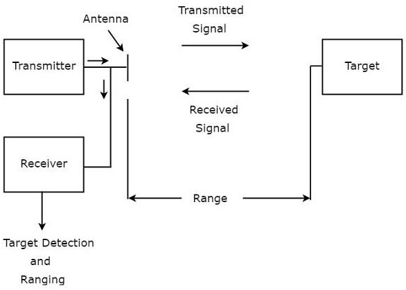
As shown in the figure, Radar mainly consists of a transmitter and a receiver. It uses the same Antenna for both transmitting and receiving the signals. The function of the transmitter is to transmit the Radar signal in the direction of the target present.
Target reflects this received signal in various directions. The signal, which is reflected back towards the Antenna gets received by the receiver.
Terminology of Radar Systems
Following are the basic terms, which are useful in this tutorial.
- Range
- Pulse Repetition Frequency
- Maximum Unambiguous Range
- Minimum Range
Now, let us discuss about these basic terms one by one.
Range
The distance between Radar and target is called Range of the target or simply range, R. We know that Radar transmits a signal to the target and accordingly the target sends an echo signal to the Radar with the speed of light, C.
Let the time taken for the signal to travel from Radar to target and back to Radar be ‘T’. The two way distance between the Radar and target will be 2R, since the distance between the Radar and the target is R.
Now, the following is the formula for Speed.
$$Speed= \frac{Distance}{Time}$$
$$\Rightarrow Distance=Speed\times Time$$
$$\Rightarrow 2R=C\times T$$
$$R=\frac{CT}{2}\:\:\:\:\:Equation\:1$$
We can find the range of the target by substituting the values of C & T in Equation 1.
Pulse Repetition Frequency
Radar signals should be transmitted at every clock pulse. The duration between the two clock pulses should be properly chosen in such a way that the echo signal corresponding to present clock pulse should be received before the next clock pulse. A typical Radar wave form is shown in the following figure.
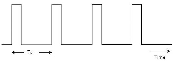
As shown in the figure, Radar transmits a periodic signal. It is having a series of narrow rectangular shaped pulses. The time interval between the successive clock pulses is called pulse repetition time, $T_P$.
The reciprocal of pulse repetition time is called pulse repetition frequency, $f_P$. Mathematically, it can be represented as
$$f_P=\frac{1}{T_P}\:\:\:\:\:Equation\:2$$Therefore, pulse repetition frequency is nothing but the frequency at which Radar transmits the signal.
Maximum Unambiguous Range
We know that Radar signals should be transmitted at every clock pulse. If we select a shorter duration between the two clock pulses, then the echo signal corresponding to present clock pulse will be received after the next clock pulse. Due to this, the range of the target seems to be smaller than the actual range.
So, we have to select the duration between the two clock pulses in such a way that the echo signal corresponding to present clock pulse will be received before the next clock pulse starts. Then, we will get the true range of the target and it is also called maximum unambiguous range of the target or simply, maximum unambiguous range.
Substitute, $R=R_{un}$ and $T=T_P$ in Equation 1.
$$R_{un}=\frac{CT_P}{2}\:\:\:\:\:Equation\:3$$
From Equation 2, we will get the pulse repetition time, $T_P$ as the reciprocal of pulse repetition frequency, $f_P$. Mathematically, it can be represented as
$$T_P=\frac{1}{f_P}\:\:\:\:\:Equation\:4$$
Substitute, Equation 4 in Equation 3.
$$R_{un}=\frac{C\left ( \frac{1}{f_P} \right )}{2}$$
$$R_{un}=\frac{C}{2f_P}\:\:\:\:\:Equation\:5$$
We can use either Equation 3 or Equation 5 for calculating maximum unambiguous range of the target.
We will get the value of maximum unambiguous range of the target, $R_{un}$ by substituting the values of $C$ and $T_P$ in Equation 3.
Similarly, we will get the value of maximum unambiguous range of the target, $R_{un}$ by substituting the values of $C$ and $f_P$ in Equation 5.
Minimum Range
We will get the minimum range of the target, when we consider the time required for the echo signal to receive at Radar after the signal being transmitted from the Radar as pulse width. It is also called the shortest range of the target.
Substitute, $R=R_{min}$ and $T=\tau$ in Equation 1.
$$R_{min}=\frac{C\tau}{2}\:\:\:\:\:Equation\:6$$
We will get the value of minimum range of the target, $R_{min}$ by substituting the values of $C$ and $\tau$ in Equation 6.
Radar Systems - Range Equation
Radar range equation is useful to know the range of the target theoretically. In this chapter, we will discuss the standard form of Radar range equation and then will discuss about the two modified forms of Radar range equation.
We will get those modified forms of Radar range equation from the standard form of Radar range equation. Now, let us discuss about the derivation of the standard form of Radar range equation.
Derivation of Radar Range Equation
The standard form of Radar range equation is also called as simple form of Radar range equation. Now, let us derive the standard form of Radar range equation.
We know that power density is nothing but the ratio of power and area. So, the power density, $P_{di}$ at a distance, R from the Radar can be mathematically represented as −
$$P_{di}=\frac{P_t}{4\pi R^2}\:\:\:\:\:Equation\:1$$
Where,
$P_t$ is the amount of power transmitted by the Radar transmitterThe above power density is valid for an isotropic Antenna. In general, Radars use directional Antennas. Therefore, the power density, $P_{dd}$ due to directional Antenna will be −
$$P_{dd}=\frac{P_tG}{4\pi R^2}\:\:\:\:\:Equation\:2$$
Target radiates the power in different directions from the received input power. The amount of power, which is reflected back towards the Radar depends on its cross section. So, the power density $P_{de}$ of echo signal at Radar can be mathematically represented as −
$$P_{de}=P_{dd}\left (\frac{\sigma}{4\pi R^2}\right )\:\:\:\:\:Equation\:3$$ Substitute, Equation 2 in Equation 3.
$$P_{de}=\left (\frac{P_tG}{4\pi R^2}\right )\left (\frac{\sigma}{4\pi R^2}\right )\:\:\:\:\:Equation\:4$$
The amount of power, $P_r$ received by the Radar depends on the effective aperture, $A_e$ of the receiving Antenna.
$$P_r=P_{de}A_e\:\:\:\:\:Equation\:5$$
Substitute, Equation 4 in Equation 5.
$$P_r=\left (\frac{P_tG}{4\pi R^2}\right )\left (\frac{\sigma}{4\pi R^2}\right )A_e$$
$$\Rightarrow P_r=\frac{P_tG\sigma A_e}{\left (4\pi\right )^2 R^4}$$
$$\Rightarrow R^4=\frac{P_tG\sigma A_e}{\left (4\pi\right )^2 P_r}$$
$$\Rightarrow R=\left [\frac{P_tG\sigma A_e}{\left (4\pi\right )^2 P_r}\right ]^{1/4}\:\:\:\:\:Equation\:6$$
Standard Form of Radar Range Equation
If the echo signal is having the power less than the power of the minimum detectable signal, then Radar cannot detect the target since it is beyond the maximum limit of the Radar's range.
Therefore, we can say that the range of the target is said to be maximum range when the received echo signal is having the power equal to that of minimum detectable signal. We will get the following equation, by substituting $R=R_{Max}$ and $P_r=S_{min}$ in Equation 6.
$$R_{Max}=\left [\frac{P_tG\sigma A_e}{\left (4\pi\right )^2 S_{min}}\right ]^{1/4}\:\:\:\:\:Equation\:7$$
Equation 7 represents the standard form of Radar range equation. By using the above equation, we can find the maximum range of the target.
Modified Forms of Radar Range Equation
We know the following relation between the Gain of directional Antenna, $G$ and effective aperture, $A_e$.
$$G=\frac{4\pi A_e}{\lambda^2}\:\:\:\:\:Equation\:8$$
Substitute, Equation 8 in Equation 7.
$$R_{Max}=\left [ \frac{P_t\sigma A_e}{\left ( 4\pi \right )^2S_{min}}\left ( \frac{4\pi A_e}{\lambda^2} \right ) \right ]^{1/4}$$
$$\Rightarrow R_{Max}=\left [\frac{P_tG\sigma {A_e}^2}{4\pi \lambda^2 S_{min}}\right ]^{1/4}\:\:\:\:\:Equation\:9$$
Equation 9 represents the modified form of Radar range equation. By using the above equation, we can find the maximum range of the target.
We will get the following relation between effective aperture, $A_e$ and the Gain of directional Antenna, $G$ from Equation 8.
$$A_e=\frac{G\lambda^2}{4\pi}\:\:\:\:\:Equation\:10$$
Substitute, Equation 10 in Equation 7.
$$R_{Max}=\left [\frac{P_tG\sigma}{\left (4\pi\right )^2 S_{min}}(\frac{G\lambda^2}{4\pi})\right ]^{1/4}$$
$$\Rightarrow R_{Max}=\left [\frac{P_tG^2 \lambda^2 \sigma}{\left (4\pi\right )^2 S_{min}}\right ]^{1/4}\:\:\:\:\:Equation\:11$$
Equation 11 represents another modified form of Radar range equation. By using the above equation, we can find the maximum range of the target.
Note − Based on the given data, we can find the maximum range of the target by using one of these three equations namely
- Equation 7
- Equation 9
- Equation 11
Example Problems
In previous section, we got the standard and modified forms of the Radar range equation. Now, let us solve a few problems by using those equations.
Problem 1
Calculate the maximum range of Radar for the following specifications −
- Peak power transmitted by the Radar, $P_t=250KW$
- Gain of transmitting Antenna, $G=4000$
- Effective aperture of the receiving Antenna, $A_e=4\:m^2$
- Radar cross section of the target, $\sigma=25\:m^2$
- Power of minimum detectable signal, $S_{min}=10^{-12}W$
Solution
We can use the following standard form of Radar range equation in order to calculate the maximum range of Radar for given specifications.
$$R_{Max}=\left [\frac{P_tG \sigma A_e}{\left (4\pi \right )^2 S_{min}}\right ]^{1/4}$$
Substitute all the given parameters in above equation.
$$R_{Max}=\left [\frac{ \left ( 250\times 10^3 \right )\left ( 4000 \right )\left ( 25 \right )\left ( 4 \right )}{\left ( 4\pi \right )^2 \left ( 10^{-12} \right )} \right ]^{1/4}$$
$$\Rightarrow R_{Max}=158\:KM$$
Therefore, the maximum range of Radar for given specifications is $158\:KM$.
Problem 2
Calculate the maximum range of Radar for the following specifications.
- Operating frequency, $f=10GHZ$
- Peak power transmitted by the Radar, $P_t=400KW$
- Effective aperture of the receiving Antenna, $A_e=5\:m^2$
- Radar cross section of the target, $\sigma=30\:m^2$
- Power of minimum detectable signal, $S_{min}=10^{-10}W$
Solution
We know the following formula for operating wavelength, $\lambda$ in terms of operating frequency, f.
$$\lambda =\frac{C}{f}$$
Substitute, $C=3\times 10^8m/sec$ and $f=10GHZ$ in above equation.
$$\lambda =\frac{3\times 10^8}{10\times 10^9}$$
$$\Rightarrow \lambda=0.03m$$
So, the operating wavelength,$\lambda$ is equal to $0.03m$, when the operating frequency, $f$ is $10GHZ$.
We can use the following modified form of Radar range equation in order to calculate the maximum range of Radar for given specifications.
$$R_{Max}=\left [\frac{P_t \sigma {A_e}^2}{4\pi \lambda^2 S_{min}}\right ]^{1/4}$$
Substitute, the given parameters in the above equation.
$$R_{Max}=\left [ \frac{\left ( 400\times 10^3 \right )\left ( 30 \right )\left ( 5^2 \right )}{4\pi\left ( 0.003 \right )^2\left ( 10 \right )^{-10}} \right ]^{1/4}$$
$$\Rightarrow R_{Max}=128KM$$
Therefore, the maximum range of Radar for given specifications is $128\:KM$.
Radar Systems - Performance Factors
The factors, which affect the performance of Radar are known as Radar performance factors. In this chapter, let us discuss about those factors. We know that the following standard form of Radar range equation, which is useful for calculating the maximum range of Radar for given specifications.
$$R_{Max}=\left [\frac{P_tG\sigma A_e}{\left (4\pi\right )^2 S_{min}}\right ]^{1/4}$$
Where,
$P_t$ is the peak power transmitted by the Radar
$G$ is the gain of transmitting Antenna
$\sigma$ is the Radar cross section of the target
$A_e$ is the effective aperture of the receiving Antenna
$S_{min}$ is the power of minimum detectable signal
From the above equation, we can conclude that the following conditions should be considered in order to get the range of the Radar as maximum.
- Peak power transmitted by the Radar $P_t$ should be high.
- Gain of the transmitting Antenna $G$ should be high.
- Radar cross section of the target $\sigma$ should be high.
- Effective aperture of the receiving Antenna $A_e$ should be high.
- Power of minimum detectable signal $S_{min}$ should be low.
It is difficult to predict the range of the target from the standard form of the Radar range equation. This means, the degree of accuracy that is provided by the Radar range equation about the range of the target is less. Because, the parameters like Radar cross section of the target, $\sigma$ and minimum detectable signal, $S_{min}$ are statistical in nature.
Minimum Detectable Signal
If the echo signal has minimum power, detecting that signal by the Radar is known as minimum detectable signal. This means, Radar cannot detect the echo signal if that signal is having less power than that of minimum power.
In general, Radar receives the echo signal in addition with noise. If the threshold value is used for detecting the presence of the target from the received signal, then that detection is called threshold detection.
We have to select proper threshold value based on the strength of the signal to be detected.
A high threshold value should be chosen when the strength of the signal to be detected is high so that it will eliminate the unwanted noise signal present in it.
Similarly, a low threshold value should be chosen when the strength of the signal to be detected is low.
The following figure illustrates this concept −
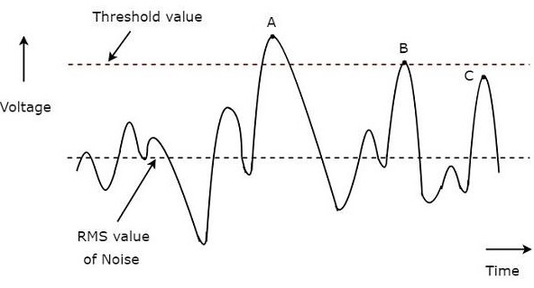
A typical waveform of the Radar receiver is shown in the above figure. The x-axis and y-axis represent time and voltage respectively. The rms value of noise and threshold value are indicated with dotted lines in the above figure.
We have considered three points, A, B & C in above figure for identifying the valid detections and missing detections.
The value of the signal at point A is greater than threshold value. Hence, it is a valid detection.
The value of the signal at point B is equal to threshold value. Hence, it is a valid detection.
Even though the value of the signal at point C is closer to threshold value, it is a missing detection. Because, the value of the signal at point C is less than threshold value.
So, the points, A & B are valid detections. Whereas, the point C is a missing detection.
Receiver Noise
If the receiver generates a noise component into the signal, which is received at the receiver, then that kind of noise is known as receiver noise. The receiver noise is an unwanted component; we should try to eliminate it with some precautions.
However, there exists one kind of noise that is known as the thermal noise. It occurs due to thermal motion of conduction electrons. Mathematically, we can write thermal noise power, $N_i$ produced at receiver as −
$$N_i=KT_oB_n$$
Where,
$K$ is the Boltzmann's constant and it is equal to $1.38\times 10^{-23}J/deg$
$T_o$ is the absolute temperature and it is equal to $290^0K$
$B_n$ is the receiver band width
Figure of Merit
The Figure of Merit, F is nothing but the ratio of input SNR, $(SNR)_i$ and output SNR, $(SNR)_o$. Mathematically, it can be represented as −
$$F=\frac{(SNR)_i}{(SNR)_o}$$
$$\Rightarrow F=\frac{S_i/N_i}{S_o/N_o}$$
$$\Rightarrow F=\frac{N_oS_i}{N_iS_o}$$
$$\Rightarrow S_i=\frac{FN_iS_o}{N_o}$$
Substitute, $N_i=KT_oB_n$ in above equation.
$$\Rightarrow S_i=FKT_oB_n\left ( \frac{S_o}{N_o}\right )$$
Input signal power will be having minimum value, when output SNR is having minimum value.
$$\Rightarrow S_{min}=FKT_oB_n\left ( \frac{S_o}{N_o}\right )_{min}$$
Substitute, the above $S_{min}$ in the following standard form of Radar range equation.
$$R_{Max}=\left [\frac{P_tG\sigma A_e}{\left (4\pi\right )^2 S_{min}}\right ]^{1/4}$$
$$\Rightarrow R_{Max}=\left [\frac{P_tG\sigma A_e}{\left (4\pi\right )^2 FKT_oB_n\left ( \frac{S_o}{N_o}\right )_{min}}\right ]^{1/4}$$
From the above equation, we can conclude that the following conditions should be considered in order to get the range of the Radar as maximum.
- Peak power transmitted by the Radar, $P_t$ should be high.
- Gain of the transmitting Antenna $G$ should be high.
- Radar cross section of the target $\sigma$ should be high.
- Effective aperture of the receiving Antenna $A_e$ should be high.
- Figure of Merit F should be low.
- Receiver bandwidth $B_n$ should be low.
Radar Systems - Types of Radars
In this chapter, we will discuss in brief the different types of Radar. This chapter provides the information briefly about the types of Radars. Radars can be classified into the following two types based on the type of signal with which Radar can be operated.
- Pulse Radar
- Continuous Wave Radar
Now, let us discuss about these two types of Radars one by one.
Pulse Radar
The Radar, which operates with pulse signal is called the Pulse Radar. Pulse Radars can be classified into the following two types based on the type of the target it detects.
- Basic Pulse Radar
- Moving Target Indication Radar
Let us now discuss the two Radars briefly.
Basic Pulse Radar
The Radar, which operates with pulse signal for detecting stationary targets, is called the Basic Pulse Radar or simply, Pulse Radar. It uses single Antenna for both transmitting and receiving signals with the help of Duplexer.
Antenna will transmit a pulse signal at every clock pulse. The duration between the two clock pulses should be chosen in such a way that the echo signal corresponding to the present clock pulse should be received before the next clock pulse.
Moving Target Indication Radar
The Radar, which operates with pulse signal for detecting non-stationary targets, is called Moving Target Indication Radar or simply, MTI Radar. It uses single Antenna for both transmission and reception of signals with the help of Duplexer.
MTI Radar uses the principle of Doppler effect for distinguishing the non-stationary targets from stationary objects.
Continuous Wave Radar
The Radar, which operates with continuous signal or wave is called Continuous Wave Radar. They use Doppler Effect for detecting non-stationary targets. Continuous Wave Radars can be classified into the following two types.
- Unmodulated Continuous Wave Radar
- Frequency Modulated Continuous Wave Radar
Now, let us discuss the two Radars briefly.
Unmodulated Continuous Wave Radar
The Radar, which operates with continuous signal (wave) for detecting non-stationary targets is called Unmodulated Continuous Wave Radar or simply, CW Radar. It is also called CW Doppler Radar.
This Radar requires two Antennas. Of these two antennas, one Antenna is used for transmitting the signal and the other Antenna is used for receiving the signal. It measures only the speed of the target but not the distance of the target from the Radar.
Frequency Modulated Continuous Wave Radar
If CW Doppler Radar uses the Frequency Modulation, then that Radar is called the Frequency Modulated Continuous Wave (FMCW) Radar or FMCW Doppler Radar. It is also called Continuous Wave Frequency Modulated Radar or CWFM Radar.
This Radar requires two Antennas. Among which, one Antenna is used for transmitting the signal and the other Antenna is used for receiving the signal. It measures not only the speed of the target but also the distance of the target from the Radar.
In our subsequent chapters, we will discuss the operations of all these Radars in detail.
Radar Systems - Pulse Radar
The Radar, which operates with pulse signal for detecting stationary targets is called Basic Pulse Radar or simply, Pulse Radar. In this chapter, let us discuss the working of Pulse Radar.
Block Diagram of Pulse Radar
Pulse Radar uses single Antenna for both transmitting and receiving of signals with the help of Duplexer. Following is the block diagram of Pulse Radar −
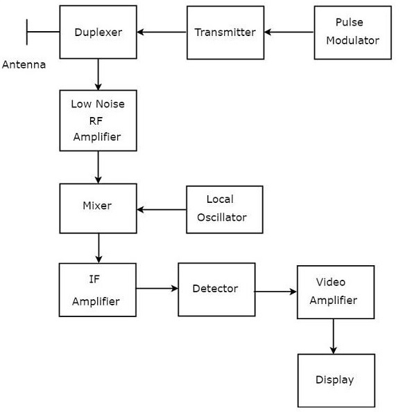
Let us now see the function of each block of Pulse Radar −
Pulse Modulator − It produces a pulse-modulated signal and it is applied to the Transmitter.
Transmitter − It transmits the pulse-modulated signal, which is a train of repetitive pulses.
Duplexer − It is a microwave switch, which connects the Antenna to both transmitter section and receiver section alternately. Antenna transmits the pulse-modulated signal, when the duplexer connects the Antenna to the transmitter. Similarly, the signal, which is received by Antenna will be given to Low Noise RF Amplifier, when the duplexer connects the Antenna to Low Noise RF Amplifier.
Low Noise RF Amplifier − It amplifies the weak RF signal, which is received by Antenna. The output of this amplifier is connected to Mixer.
Local Oscillator − It produces a signal having stable frequency. The output of Local Oscillator is connected to Mixer.
Mixer − We know that Mixer can produce both sum and difference of the frequencies that are applied to it. Among which, the difference of the frequencies will be of Intermediate Frequency (IF) type.
IF Amplifier − IF amplifier amplifies the Intermediate Frequency (IF) signal. The IF amplifier shown in the figure allows only the Intermediate Frequency, which is obtained from Mixer and amplifies it. It improves the Signal to Noise Ratio at output.
Detector − It demodulates the signal, which is obtained at the output of the IF Amplifier.
Video Amplifier − As the name suggests, it amplifies the video signal, which is obtained at the output of detector.
Display − In general, it displays the amplified video signal on CRT screen.
In this chapter, we discussed how the Pulse Radar works and how it is useful for detecting stationary targets. In our subsequent chapters, we will discuss the Radars, which are useful for detecting non-stationary targets.
Radar Systems - Doppler Effect
In this chapter, we will learn about the Doppler Effect in Radar Systems.
If the target is not stationary, then there will be a change in the frequency of the signal that is transmitted from the Radar and that is received by the Radar. This effect is known as the Doppler effect.
According to the Doppler effect, we will get the following two possible cases −
The frequency of the received signal will increase, when the target moves towards the direction of the Radar.
The frequency of the received signal will decrease, when the target moves away from the Radar.
Now, let us derive the formula for Doppler frequency.
Derivation of Doppler Frequency
The distance between Radar and target is nothing but the Range of the target or simply range, R. Therefore, the total distance between the Radar and target in a two-way communication path will be 2R, since Radar transmits a signal to the target and accordingly the target sends an echo signal to the Radar.
If $\lambda$ is one wave length, then the number of wave lengths N that are present in a two-way communication path between the Radar and target will be equal to $2R/\lambda$.
We know that one wave length $\lambda$ corresponds to an angular excursion of $2\pi$ radians. So, the total angle of excursion made by the electromagnetic wave during the two-way communication path between the Radar and target will be equal to $4\pi R/\lambda$ radians.
Following is the mathematical formula for angular frequency, $\omega$ −
$$\omega=2\pi f\:\:\:\:\:Equation\:1$$
Following equation shows the mathematical relationship between the angular frequency $\omega$ and phase angle $\phi$ −
$$\omega=\frac{d\phi }{dt}\:\:\:\:\:Equation\:2$$
Equate the right hand side terms of Equation 1 and Equation 2 since the left hand side terms of those two equations are same.
$$2\pi f=\frac{d\phi }{dt}$$
$$\Rightarrow f =\frac{1}{2\pi}\frac{d\phi }{dt}\:\:\:\:\:Equation\:3$$
Substitute,$f=f_d$ and $\phi=4\pi R/\lambda$ in Equation 3.
$$f_d =\frac{1}{2\pi}\frac{d}{dt}\left ( \frac{4\pi R}{\lambda} \right )$$
$$\Rightarrow f_d =\frac{1}{2\pi}\frac{4\pi}{\lambda}\frac{dR}{dt}$$
$$\Rightarrow f_d =\frac{2V_r}{\lambda}\:\:\:\:\:Equation\:4$$
Where,
$f_d$ is the Doppler frequency
$V_r$ is the relative velocity
We can find the value of Doppler frequency $f_d$ by substituting the values of $V_r$ and $\lambda$ in Equation 4.
Substitute, $\lambda=C/f$ in Equation 4.
$$f_d =\frac{2V_r}{C/f}$$
$$\Rightarrow f_d =\frac{2V_rf}{C}\:\:\:\:\:Equation\:5$$
Where,
$f$ is the frequency of transmitted signal
$C$ is the speed of light and it is equal to $3\times 10^8m/sec$
We can find the value of Doppler frequency, $f_d$ by substituting the values of $V_r,f$ and $C$ in Equation 5.
Note − Both Equation 4 and Equation 5 show the formulae of Doppler frequency, $f_d$. We can use either Equation 4 or Equation 5 for finding Doppler frequency, $f_d$ based on the given data.
Example Problem
If the Radar operates at a frequency of $5GHZ$, then find the Doppler frequency of an aircraft moving with a speed of 100KMph.
Solution
Given,
The frequency of transmitted signal, $f=5GHZ$
Speed of aircraft (target), $V_r=100KMph$
$$\Rightarrow V_r=\frac{100\times 10^3}{3600}m/sec$$
$$\Rightarrow V_r=27.78m/sec$$
We have converted the given speed of aircraft (target), which is present in KMph into its equivalent m/sec.
We know that, the speed of the light, $C=3\times 10^8m/sec$
Now, following is the formula for Doppler frequency −
$$f_d=\frac{2Vrf}{C}$$
Substitute the values of ð‘‰ð‘Ÿ, $V_r,f$ and $C$ in the above equation.
$$\Rightarrow f_d=\frac{2\left ( 27.78 \right )\left ( 5\times 10^9 \right )}{3\times 10^8}$$
$$\Rightarrow f_d=926HZ$$
Therefore, the value of Doppler frequency, $f_d$ is $926HZ$ for the given specifications.
Radar Systems - CW Radar
basic Radar uses the same Antenna for both transmission and reception of signals. We can use this type of Radar, when the target is stationary, i.e., not moving and / or when that Radar can be operated with pulse signal.
The Radar, which operates with continuous signal (wave) for detecting non-stationary targets, is called Continuous Wave Radar or simply CW Radar. This Radar requires two Antennas. Among which, one Antenna is used for transmitting the signal and the other Antenna is used for receiving the signal.
Block Diagram of CW Radar
We know that CW Doppler Radar contains two Antennas − transmitting Antenna and receiving Antenna. Following figure shows the block diagram of CW Radar −
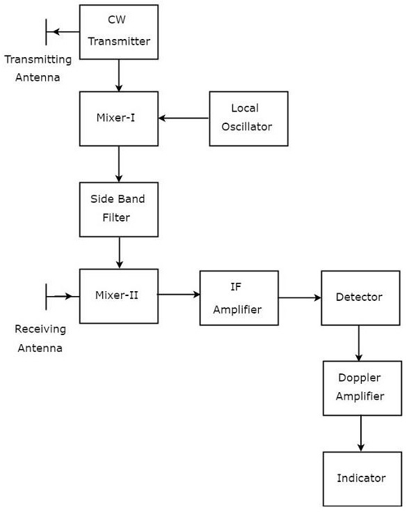
The block diagram of CW Doppler Radar contains a set of blocks and the function of each block is mentioned below.
CW Transmitter − It produces an analog signal having a frequency of $f_o$. The output of CW Transmitter is connected to both transmitting Antenna and Mixer-I.
Local Oscillator − It produces a signal having a frequency of $f_l$. The output of Local Oscillator is connected to Mixer-I.
Mixer-I − Mixer can produce both sum and difference of the frequencies that are applied to it. The signals having frequencies of $f_o$ and $f_l$ are applied to Mixer-I. So, the Mixer-I will produce the output having frequencies $f_o+f_l$ or $f_o−f_l$.
Side Band Filter − As the name suggests, side band filter allows a particular side band frequencies − either upper side band frequencies or lower side band frequencies. The side band filter shown in the above figure produces only upper side band frequency, i.e., $f_o+f_l$.
Mixer-II − Mixer can produce both sum and difference of the frequencies that are applied to it. The signals having frequencies of $f_o+f_l$ and $f_o\pm f_d$ are applied to Mixer-II. So, the Mixer-II will produce the output having frequencies of 2$f_o+f_l\pm f_d$ or $f_l\pm f_d$.
IF Amplifier − IF amplifier amplifies the Intermediate Frequency (IF) signal. The IF amplifier shown in the figure allows only the Intermediate Frequency, $f_l\pm f_d$ and amplifies it.
Detector − It detects the signal, which is having Doppler frequency, $f_d$.
Doppler Amplifier − As the name suggests, Doppler amplifier amplifies the signal, which is having Doppler frequency, $f_d$.
Indicator − It indicates the information related relative velocity and whether the target is inbound or outbound.
CW Doppler Radars give accurate measurement of relative velocities. Hence, these are used mostly, where the information of velocity is more important than the actual range.
Radar Systems - FMCW Radar
If CW Doppler Radar uses the Frequency Modulation, then that Radar is called FMCW Doppler Radar or simply, FMCW Radar. It is also called Continuous Wave Frequency Modulated Radar or CWFM Radar. It measures not only the speed of the target but also the distance of the target from the Radar.
Block Diagram of FMCW Radar
FMCW Radar is mostly used as Radar Altimeter in order to measure the exact height while landing the aircraft. The following figure shows the block diagram of FMCW Radar −
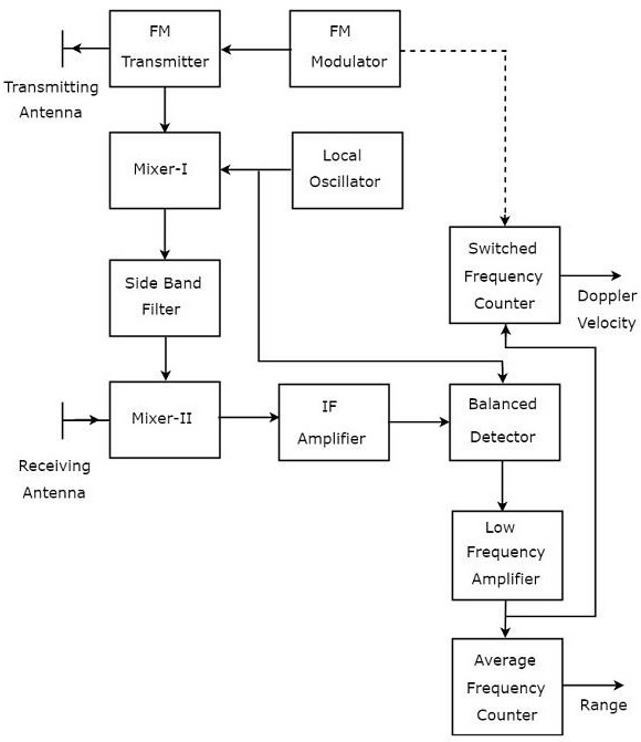
FMCW Radar contains two Antennas − transmitting Antenna and receiving Antenna as shown in the figure. The transmitting Antenna transmits the signal and the receiving Antenna receives the echo signal.
The block diagram of the FMCW Radar looks similar to the block diagram of CW Radar. It contains few modified blocks and some other blocks in addition to the blocks that are present in the block diagram of CW Radar. The function of each block of FMCW Radar is mentioned below.
FM Modulator − It produces a Frequency Modulated (FM) signal having variable frequency, $f_o\left (t \right )$ and it is applied to the FM transmitter.
FM Transmitter − It transmits the FM signal with the help of transmitting Antenna. The output of FM Transmitter is also connected to Mixer-I.
Local Oscillator − In general, Local Oscillator is used to produce an RF signal. But, here it is used to produce a signal having an Intermediate Frequency, $f_{IF}$. The output of Local Oscillator is connected to both Mixer-I and Balanced Detector.
Mixer-I − Mixer can produce both sum and difference of the frequencies that are applied to it. The signals having frequencies of $f_o\left (t \right )$ and $f_{IF}$ are applied to Mixer-I. So, the Mixer-I will produce the output having frequency either $f_o\left (t \right )+f_{IF}$ or $f_o\left (t \right )-f_{IF}$.
Side Band Filter − It allows only one side band frequencies, i.e., either upper side band frequencies or lower side band frequencies. The side band filter shown in the figure produces only lower side band frequency. i.e., $f_o\left (t \right )-f_{IF}$.
Mixer-II − Mixer can produce both sum and difference of the frequencies that are applied to it. The signals having frequencies of $f_o\left (t \right )-f_{IF}$ and $f_o\left (t-T \right )$ are applied to Mixer-II. So, the Mixer-II will produce the output having frequency either $f_o\left (t-T \right )+f_o\left (t \right )-f_{IF}$ or $f_o\left (t-T \right )-f_o\left (t \right )+f_{IF}$.
IF Amplifier − IF amplifier amplifies the Intermediate Frequency (IF) signal. The IF amplifier shown in the figure amplifies the signal having frequency of $f_o\left (t-T \right )-f_o\left (t \right )+f_{IF}$. This amplified signal is applied as an input to the Balanced detector.
Balanced Detector − It is used to produce the output signal having frequency of $f_o\left (t-T \right )-f_o\left (t \right )$ from the applied two input signals, which are having frequencies of $f_o\left (t-T \right )-f_o\left (t \right )+f_{IF}$ and $f_{IF}$. The output of Balanced detector is applied as an input to Low Frequency Amplifier.
Low Frequency Amplifier − It amplifies the output of Balanced detector to the required level. The output of Low Frequency Amplifier is applied to both switched frequency counter and average frequency counter.
Switched Frequency Counter − It is useful for getting the value of Doppler velocity.
Average Frequency Counter − It is useful for getting the value of Range.
Radar Systems - MTI Radar
If the Radar is used for detecting the movable target, then the Radar should receive only the echo signal due to that movable target. This echo signal is the desired one. However, in practical applications, Radar receives the echo signals due to stationary objects in addition to the echo signal due to that movable target.
The echo signals due to stationary objects (places) such as land and sea are called clutters because these are unwanted signals. Therefore, we have to choose the Radar in such a way that it considers only the echo signal due to movable target but not the clutters.
For this purpose, Radar uses the principle of Doppler Effect for distinguishing the non-stationary targets from stationary objects. This type of Radar is called Moving Target Indicator Radar or simply, MTI Radar.
According to Doppler effect, the frequency of the received signal will increase if the target is moving towards the direction of Radar. Similarly, the frequency of the received signal will decrease if the target is moving away from the Radar.
Types of MTI Radars
We can classify the MTI Radars into the following two types based on the type of transmitter that has been used.
- MTI Radar with Power Amplifier Transmitter
- MTI Radar with Power Oscillator Transmitter
Now, let us discuss about these two MTI Radars one by one.
MTI Radar with Power Amplifier Transmitter
MTI Radar uses single Antenna for both transmission and reception of signals with the help of Duplexer. The block diagram of MTI Radar with power amplifier transmitter is shown in the following figure.
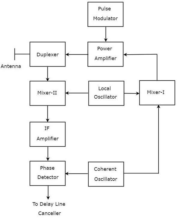
The function of each block of MTI Radar with power amplifier transmitter is mentioned below.
Pulse Modulator − It produces a pulse modulated signal and it is applied to Power Amplifier.
Power Amplifier − It amplifies the power levels of the pulse modulated signal.
Local Oscillator − It produces a signal having stable frequency $f_l$. Hence, it is also called stable Local Oscillator. The output of Local Oscillator is applied to both Mixer-I and Mixer-II.
Coherent Oscillator − It produces a signal having an Intermediate Frequency, $f_c$. This signal is used as the reference signal. The output of Coherent Oscillator is applied to both Mixer-I and Phase Detector.
Mixer-I − Mixer can produce either sum or difference of the frequencies that are applied to it. The signals having frequencies of $f_l$ and $f_c$ are applied to Mixer-I. Here, the Mixer-I is used for producing the output, which is having the frequency $f_l+f_c$.
Duplexer − It is a microwave switch, which connects the Antenna to either the transmitter section or the receiver section based on the requirement. Antenna transmits the signal having frequency $f_l+f_c$ when the duplexer connects the Antenna to power amplifier. Similarly, Antenna receives the signal having frequency of $f_l+f_c\pm f_d$ when the duplexer connects the Antenna to Mixer-II.
Mixer-II − Mixer can produce either sum or difference of the frequencies that are applied to it. The signals having frequencies $f_l+f_c\pm f_d$ and $f_l$ are applied to Mixer-II. Here, the Mixer-II is used for producing the output, which is having the frequency $f_c\pm f_d$.
IF Amplifier − IF amplifier amplifies the Intermediate Frequency (IF) signal. The IF amplifier shown in the figure amplifies the signal having frequency $f_c+f_d$. This amplified signal is applied as an input to Phase detector.
Phase Detector − It is used to produce the output signal having frequency $f_d$ from the applied two input signals, which are having the frequencies of $f_c+f_d$ and $f_c$. The output of phase detector can be connected to Delay line canceller.
MTI Radar with Power Oscillator Transmitter
The block diagram of MTI Radar with power oscillator transmitter looks similar to the block diagram of MTI Radar with power amplifier transmitter. The blocks corresponding to the receiver section will be same in both the block diagrams. Whereas, the blocks corresponding to the transmitter section may differ in both the block diagrams.
The block diagram of MTI Radar with power oscillator transmitter is shown in the following figure.
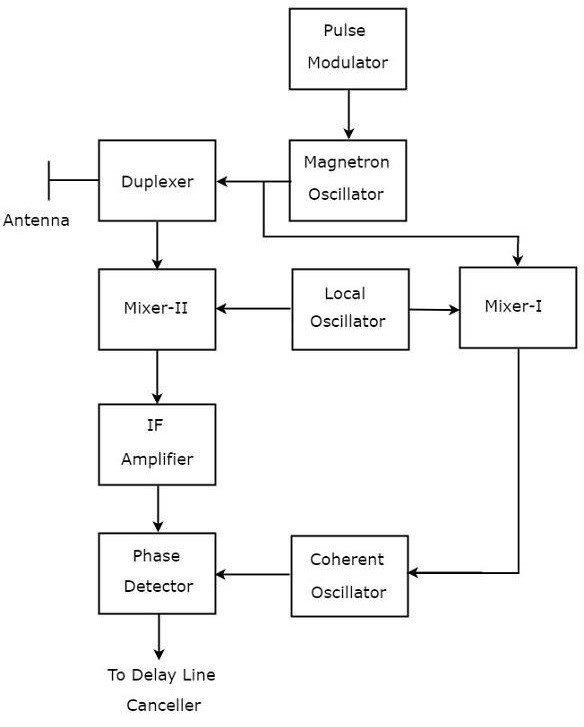
As shown in the figure, MTI Radar uses the single Antenna for both transmission and reception of signals with the help of Duplexer. The operation of MTI Radar with power oscillator transmitter is mentioned below.
The output of Magnetron Oscillator and the output of Local Oscillator are applied to Mixer-I. This will further produce an IF signal, the phase of which is directly related to the phase of the transmitted signal.
The output of Mixer-I is applied to the Coherent Oscillator. Therefore, the phase of Coherent Oscillator output will be locked to the phase of IF signal. This means, the phase of Coherent Oscillator output will also directly relate to the phase of the transmitted signal.
So, the output of Coherent Oscillator can be used as reference signal for comparing the received echo signal with the corresponding transmitted signal using phase detector.
The above tasks will be repeated for every newly transmitted signal.
Radar Systems - Delay Line Cancellers
In this chapter, we will learn about Delay Line Cancellers in Radar Systems. As the name suggests, delay line introduces a certain amount of delay. So, the delay line is mainly used in Delay line canceller in order to introduce a delay of pulse repetition time.
Delay line canceller is a filter, which eliminates the DC components of echo signals received from stationary targets. This means, it allows the AC components of echo signals received from non-stationary targets, i.e., moving targets.
Types of Delay Line Cancellers
Delay line cancellers can be classified into the following two types based on the number of delay lines that are present in it.
- Single Delay Line Canceller
- Double Delay Line Canceller
In our subsequent sections, we will discuss more about these two Delay line cancellers.
Single Delay Line Canceller
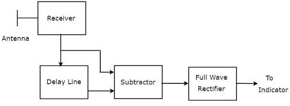
The combination of a delay line and a subtractor is known as Delay line canceller. It is also called single Delay line canceller. The block diagram of MTI receiver with single Delay line canceller is shown in the figure below.
We can write the mathematical equation of the received echo signal after the Doppler effect as −
$$V_1=A\sin\left [ 2\pi f_dt-\phi_0 \right ]\:\:\:\:\:Equation\:1$$
Where,
A is the amplitude of video signal
$f_d$ is the Doppler frequency
$\phi_o$ is the phase shift and it is equal to $4\pi f_tR_o/C$
We will get the output of Delay line canceller, by replacing $t$ by $t-T_P$ in Equation 1.
$$V_2=A\sin\left [ 2\pi f_d\left ( t-T_P\right )-\phi_0 \right ]\:\:\:\:\:Equation\:2$$
Where,
$T_P$ is the pulse repetition time
We will get the subtractor output by subtracting Equation 2 from Equation 1.
$$V_1-V_2=A\sin\left [ 2\pi f_dt-\phi_0 \right ]-A\sin\left [ 2\pi f_d\left ( t-T_P\right )-\phi_0 \right ]$$
$$\Rightarrow V_1-V_2=2A\sin\left [ \frac{ 2\pi f_dt-\phi_0-\left [ 2\pi f_d\left ( t-T_P \right )-\phi_0 \right ]}{2}\right ]\cos\left [ \frac{ 2\pi f_dt-\phi_o+2\pi f_d\left ( t-T_P \right )-\phi_0 }{2}\right ]$$
$$V_1-V_2=2A\sin\left [ \frac{2\pi f_dT_P}{2} \right ]\cos\left [ \frac{2\pi f_d\left ( 2t-T_P \right )-2\phi_0}{2} \right ]$$
$$\Rightarrow V_1-V_2=2A\sin\left [ \pi f_dT_p \right ]\cos\left [ 2\pi f_d\left ( t-\frac{T_P}{2} \right )-\phi_0 \right ]\:\:\:\:\:Equation\:3$$
The output of subtractor is applied as input to Full Wave Rectifier. Therefore, the output of Full Wave Rectifier looks like as shown in the following figure. It is nothing but the frequency response of the single delay line canceller.
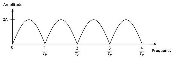
From Equation 3, we can observe that the frequency response of the single delay line canceller becomes zero, when $\pi f_dT_P$ is equal to integer multiples of $\pi$ This means, $\pi f_dT_P$ is equal to $n\pi$ Mathematically, it can be written as
$$\pi f_dT_P=n\pi$$
$$\Rightarrow f_dT_P=n$$
$$\Rightarrow f_d=\frac{n}{T_P}\:\:\:\:\:Equation\:4$$
From Equation 4, we can conclude that the frequency response of the single delay line canceller becomes zero, when Doppler frequency $f_d$ is equal to integer multiples of reciprocal of pulse repetition time $T_P$.
We know the following relation between the pulse repetition time and pulse repetition frequency.
$$f_d=\frac{1}{T_P}$$
$$\Rightarrow \frac{1}{T_P}=f_P\:\:\:\:\:Equation\:5$$
We will get the following equation, by substituting Equation 5 in Equation 4.
$$\Rightarrow f_d=nf_P\:\:\:\:\:Equation\:6$$
From Equation 6, we can conclude that the frequency response of the single delay line canceller becomes zero, when Doppler frequency, $f_d$ is equal to integer multiples of pulse repetition frequency $f_P$.
Blind Speeds
From what we learnt so far, single Delay line canceller eliminates the DC components of echo signals received from stationary targets, when $n$ is equal to zero. In addition to that, it also eliminates the AC components of echo signals received from non-stationary targets, when the Doppler frequency $f_d$ is equal to integer (other than zero) multiples of pulse repetition frequency $f_P$.
So, the relative velocities for which the frequency response of the single delay line canceller becomes zero are called blind speeds. Mathematically, we can write the expression for blind speed $v_n$ as −
$$v_n=\frac{n\lambda}{2T_P}\:\:\:\:\:Equation\:7$$
$$\Rightarrow v_n=\frac{n\lambda f_P}{2}\:\:\:\:\:Equation\:8$$
Where,
$n$ is an integer and it is equal to 1, 2, 3 and so on
$\lambda$ is the operating wavelength
Example Problem
An MTI Radar operates at a frequency of $6GHZ$ with a pulse repetition frequency of $1KHZ$. Find the first, second and third blind speeds of this Radar.
Solution
Given,
The operating frequency of MTI Radar, $f=6GHZ$
Pulse repetition frequency, $f_P=1KHZ$.
Following is the formula for operating wavelength $\lambda$ in terms of operating frequency, f.
$$\lambda=\frac{C}{f}$$
Substitute, $C=3\times10^8m/sec$ and $f=6GHZ$ in the above equation.
$$\lambda=\frac{3\times10^8}{6\times10^9}$$
$$\Rightarrow \lambda=0.05m$$
So, the operating wavelength $\lambda$ is equal to $0.05m$, when the operating frequency f is $6GHZ$.
We know the following formula for blind speed.
$$v_n=\frac{n\lambda f_p}{2}$$
By substituting, $n$=1,2 & 3 in the above equation, we will get the following equations for first, second & third blind speeds respectively.
$$v_1=\frac{1\times \lambda f_p}{2}=\frac{\lambda f_p}{2}$$
$$v_2=\frac{2\times \lambda f_p}{2}=2\left ( \frac{\lambda f_p}{2} \right )=2v_1$$
$$v_3=\frac{3\times \lambda f_p}{2}=3\left ( \frac{\lambda f_p}{2} \right )=3v_1$$
Substitute the values of $\lambda$ and $f_P$ in the equation of first blind speed.
$$v_1=\frac{0.05\times 10^3}{2}$$
$$\Rightarrow v_1=25m/sec$$
Therefore, the first blind speed $v_1$ is equal to $25m/sec$ for the given specifications.
We will get the values of second & third blind speeds as $50m/sec$& $75m/sec$ respectively by substituting the value of ð‘£1 in the equations of second & third blind speeds.
Double Delay Line Canceller
We know that a single delay line canceller consists of a delay line and a subtractor. If two such delay line cancellers are cascaded together, then that combination is called Double delay line canceller. The block diagram of Double delay line canceller is shown in the following figure.
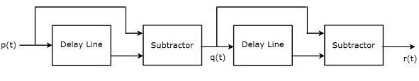
Let $p\left ( t \right )$ and $q\left ( t \right )$ be the input and output of the first delay line canceller. We will get the following mathematical relation from first delay line canceller.
$$q\left ( t \right )=p\left ( t \right )-p\left ( t-T_P \right )\:\:\:\:\:Equation\:9$$
The output of the first delay line canceller is applied as an input to the second delay line canceller. Hence, $q\left ( t \right )$ will be the input of the second delay line canceller. Let $r\left ( t \right )$ be the output of the second delay line canceller. We will get the following mathematical relation from the second delay line canceller.
$$r\left ( t \right )=q\left ( t \right )-q\left ( t-T_P \right )\:\:\:\:\:Equation\:10$$
Replace $t$ by $t-T_P$ in Equation 9.
$$q\left ( t-T_P \right )=p\left ( t-T_P \right )-p\left ( t-T_P-T_P \right )$$
$$q\left ( t-T_P \right )=p\left ( t-T_P \right )-p\left ( t-2T_P \right )\:\:\:\:\:Equation\:11$$
Substitute, Equation 9 and Equation 11 in Equation 10.
$$r\left ( t \right )=p\left ( t \right )-p\left ( t-T_P \right )-\left [ p\left ( t-T_P \right )-p\left ( t-2T_P \right ) \right ]$$
$$\Rightarrow r\left ( t \right )=p\left ( t \right )-2p\left ( t-T_P \right )+p\left ( t-2T_P \right )\:\:\:\:\:Equation\:12$$
The advantage of double delay line canceller is that it rejects the clutter broadly. The output of two delay line cancellers, which are cascaded, will be equal to the square of the output of single delay line canceller.
So, the magnitude of output of double delay line canceller, which is present at MTI Radar receiver will be equal to $4A^2\left ( \sin\left [ \pi f_dT_P \right ] \right )^2$.
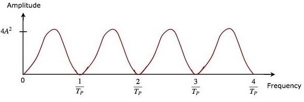
The frequency response characteristics of both double delay line canceller and the cascaded combination of two delay line cancellers are the same. The advantage of time domain delay line canceller is that it can be operated for all frequency ranges.
Radar Systems - Tracking Radar
The Radar, which is used to track the path of one or more targets is known as Tracking Radar. In general, it performs the following functions before it starts the tracking activity.
- Target detection
- Range of the target
- Finding elevation and azimuth angles
- Finding Doppler frequency shift
So, Tracking Radar tracks the target by tracking one of the three parameters — range, angle, Doppler frequency shift. Most of the Tracking Radars use the principle of tracking in angle. Now, let us discuss what angular tracking is.
Angular Tracking
The pencil beams of Radar Antenna perform tracking in angle. The axis of Radar Antenna is considered as the reference direction. If the direction of the target and reference direction is not same, then there will be angular error, which is nothing but the difference between the two directions.
If the angular error signal is applied to a servo control system, then it will move the axis of the Radar Antenna towards the direction of target. Both the axis of Radar Antenna and the direction of target will coincide when the angular error is zero. There exists a feedback mechanism in the Tracking Radar, which works until the angular error becomes zero.
Following are the two techniques, which are used in angular tracking.
- Sequential Lobing
- Conical Scanning
Now, let us discuss about these two techniques one by one.
Sequential Lobing
If the Antenna beams are switched between two patterns alternately for tracking the target, then it is called sequential lobing. It is also called sequential switching and lobe switching. This technique is used to find the angular error in one coordinate. It gives the details of both magnitude and direction of angular error.
Following figure shows an example of sequential lobing in polar coordinates.
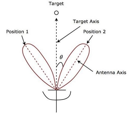
As shown in the figure, Antenna beams switch between Position 1 and Position 2 alternately. Angular error θ is indicated in the above figure. Sequential lobing gives the position of the target with high accuracy. This is the main advantage of sequential lobing.
Conical Scanning
If the Antenna beam continuously rotates for tracking a target, then it is called conical scanning. Conical scan modulation is used to find the position of the target. Following figure shows an example of conical scanning.
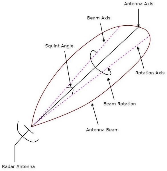
Squint angle is the angle between beam axis and rotation axis and it is shown in the above figure. The echo signal obtained from the target gets modulated at a frequency equal to the frequency at which the Antenna beam rotates.
The angle between the direction of the target and the rotation axis determines the amplitude of the modulated signal. So, the conical scan modulation has to be extracted from the echo signal and then it is to be applied to servo control system, which moves the Antenna beam axis towards the direction of the target.
Radar Systems - Antenna Parameters
An Antenna or Aerial is a transducer, which converts electrical power into electromagnetic waves and vice versa.
An Antenna has the following parameters −
- Directivity
- Aperture Efficiency
- Antenna Efficiency
- Gain
Now, let us discuss these parameters in detail −
Directivity
According to the standard definition, “The ratio of maximum radiation intensity of the subject Antenna to the radiation intensity of an isotropic or reference Antenna, radiating the same total power is called the Directivity.”
Though an Antenna radiates power, the direction in which it radiates matters is of much significance. The Antenna under study is termed as subject Antenna. Its radiation intensity is focused in a particular direction, while it is transmitting or receiving. Hence, the Antenna is said to have its directivity in that particular direction.
The ratio of radiation intensity in a given direction from an Antenna to the radiation intensity averaged over all directions, is termed as Directivity.
If that particular direction is not specified, then the direction in which maximum intensity is observed, can be taken as the directivity of that Antenna.
The directivity of a non-isotropic Antenna is equal to the ratio of the radiation intensity in a given direction to the radiation intensity of the isotropic source.
Mathematically, we can write the expression for Directivity as −
$$Directivity=\frac{U_{Max}\left (\theta,\phi\right )}{U_0}$$
Where,
$U_{Max}\left (\theta,\phi\right )$ is the maximum radiation intensity of subject Antenna
$U_0$ is the radiation intensity of an isotropic Antenna.
Aperture Efficiency
According to the standard definition, “Aperture efficiency of an Antenna is the ratio of the effective radiating area (or effective area) to the physical area of the aperture.”
An Antenna radiates power through an aperture. This radiation should be effective with minimum losses. The physical area of the aperture should also be taken into consideration, as the effectiveness of the radiation depends upon the area of the aperture, physically on the Antenna.
Mathematically, we can write the expression for Aperture efficiency $\epsilon_A$ as
$$\epsilon _A=\frac{A_{eff}}{A_p}$$
Where,
$A_{eff}$ is the effective area
$A_P$ is the physical area
Antenna Efficiency
According to the standard definition, “Antenna Efficiency is the ratio of the radiated power of the Antenna to the input power accepted by the Antenna.”
Any Antenna is designed to radiate power with minimum losses, for a given input. The efficiency of an Antenna explains how much an Antenna is able to deliver its output effectively with minimum losses in the transmission line. It is also called Radiation Efficiency Factor of the Antenna.
Mathematically, we can write the expression for Antenna efficiency 𝜂𝑒 as −
$$\eta _e=\frac{P_{Rad}}{P_{in}}$$
Where,
$P_{Rad}$ is the amount of power radiated
$P_{in}$ is the input power for the Antenna
Gain
According to the standard definition, “Gain of an Antenna is the ratio of the radiation intensity in a given direction to the radiation intensity that would be obtained if the power accepted by the Antenna were radiated isotropically.”
Simply, Gain of an Antenna takes the Directivity of Antenna into account along with its effective performance. If the power accepted by the Antenna was radiated isotropically (that means in all directions), then the radiation intensity we get can be taken as a referential.
The term Antenna gain describes how much power is transmitted in the direction of peak radiation to that of an isotropic source.
Gain is usually measured in dB.
Unlike Directivity, Antenna gain takes the losses that occur also into account and hence focuses on the efficiency.
Mathematically, we can write the expression for Antenna Gain $G$ as −
$$G=\eta_eD$$
Where,
$\eta_e$ is the Antenna efficiency
$D$ is the Directivity of the Antenna
Radar Systems - Radar Antennas
In this chapter, let us learn about the Antennas, which are useful in Radar communication. We can classify the Radar Antennas into the following two types based on the physical structure.
- Parabolic Reflector Antennas
- Lens Antennas
In our subsequent sections, we will discuss the two types of Antennas in detail.
Parabolic Reflector Antennas
Parabolic Reflector Antennas are the Microwave Antennas. A knowledge of parabolic reflector is essential to understand about working of antennas in depth.
Principle of Operation
Parabola is nothing but the Locus of points, which move in such a way that its distance from the fixed point (called focus) plus its distance from a straight line (called directrix) is constant.
The following figure shows the geometry of parabolic reflector. The points F and V are the focus (feed is given) and the vertex respectively. The line joining F and V is the axis of symmetry. $P_1Q_1, P_2Q_2$ and $P_3Q_3$ are the reflected rays. The line L represents the directrix on which the reflected points lie (to say that they are being collinear).
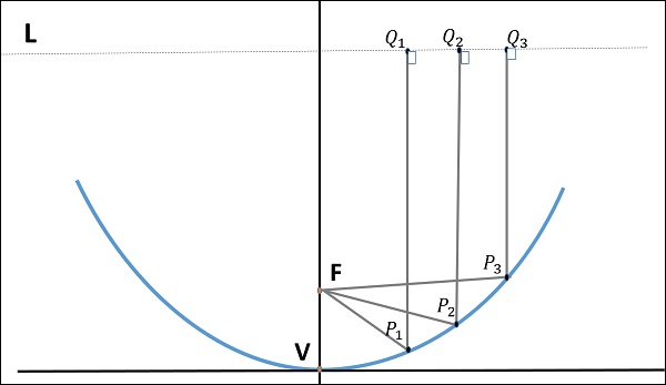
As shown in the figure, the distance between F and L lie constant with respect to the waves being focussed. The reflected wave forms a collimated wave front, out of the parabolic shape. The ratio of focal length to aperture size (i.e., $f/D$ ) is known as “f over D ratio”. It is an important parameter of parabolic reflector and its value varies from 0.25 to 0.50.
The law of reflection states that the angle of incidence and the angle of reflection are equal. This law when used along with a parabola helps the beam focus. The shape of the parabola when used for the purpose of reflection of waves, exhibits some properties of the parabola, which are helpful for building an Antenna, using the waves reflected.
Properties of Parabola
Following are the different properties of Parabola −
All the waves originating from focus reflect back to the parabolic axis. Hence, all the waves reaching the aperture are in phase.
As the waves are in phase, the beam of radiation along the parabolic axis will be strong and concentrated.
Following these points, the parabolic reflectors help in producing high directivity with narrower beam width.
Construction & Working of a Parabolic Reflector
If a Parabolic Reflector Antenna is used for transmitting a signal, the signal from the feed comes out of a dipole Antenna or horn Antenna, to focus the wave on to the parabola. It means that, the waves come out of the focal point and strike the paraboloid reflector. This wave now gets reflected as collimated wave front, as discussed previously, to get transmitted.
The same Antenna is used as a receiver. When the electromagnetic wave hits the shape of the parabola, the wave gets reflected onto the feed point. The dipole Antenna or the horn Antenna, which acts as the receiver Antenna at its feed receives this signal, to convert it into electric signal and forwards it to the receiver circuitry.
The gain of the paraboloid is a function of aperture ratio $D/\lambda$. The Effective Radiated Power (ERP) of an Antenna is the multiplication of the input power fed to the Antenna and its power gain.
Usually a wave guide horn Antenna is used as a feed radiator for the paraboloid reflector Antenna. Along with this technique, we have the following two types of feeds given to the paraboloid reflector Antenna.
- Cassegrain Feed
- Gregorian Feed
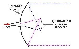
Cassegrain Feed
In this type, the feed is located at the vertex of the paraboloid, unlike in the parabolic reflector. A convex shaped reflector, which acts as a hyperboloid is placed opposite to the feed of the Antenna. It is also known as secondary hyperboloid reflector or sub-reflector. It is placed in such a way that one of its foci coincides with the focus of the paraboloid. Thus, the wave gets reflected twice.
The above figure shows the working model of the cassegrain feed.
Gregorian Feed
The type of feed where a pair of certain configurations are there and where the feed beam width is progressively increased while Antenna dimensions are held fixed is known as Gregorian feed. Here, the convex shaped hyperboloid of Cassegrain is replaced with a concave shaped paraboloid reflector, which is of course, smaller in size.
These Gregorian feed type reflectors can be used in the following four ways −
Gregorian systems using reflector ellipsoidal sub-reflector at foci F1.
Gregorian systems using reflector ellipsoidal sub-reflector at foci F2.
Cassegrain systems using hyperboloid sub-reflector (convex).
Cassegrain systems using hyperboloid sub-reflector (concave but the feed being very near to it).
Among the different types of reflector Antennas, the simple parabolic reflectors and the Cassegrain feed parabolic reflectors are the most commonly used ones.
Lens Antennas
Lens Antennas use the curved surface for both transmission and reception of signals. These antennas are made up of glass, where the converging and diverging properties of lens are followed. The frequency range of usage of Lens Antenna starts at 1 GHz but its use is greater at 3 GHz and above.
A knowledge of Lens is required to understand the working of Lens Antenna in depth. Recall that a normal glass Lens works on the principle of refraction.
Construction & Working of Lens Antenna
If a light source is assumed to be present at a focal point of a lens, which is at a focal distance from the Lens, then the rays get through the Lens as collimated or parallel rays on the plane wave front.
There are two phenomena that happens when rays fall from different sides of a lens. They are given here −
The rays that pass through the centre of the Lens are less refracted than the rays that pass through the edges of the Lens. All of the rays are sent in parallel to the plane wave front. This phenomenon of Lens is called as Divergence.
The same procedure gets reversed if a light beam is sent from the right side to the left side of the same Lens. Then the beam gets refracted and meets at a point called the focal point, at a focal distance from the Lens. This phenomenon is called Convergence.
The following diagram will help us understand the phenomenon better.
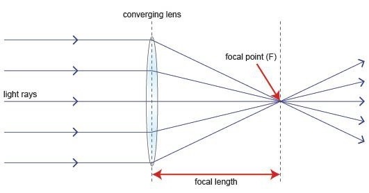
The ray diagram represents the focal point and the focal length from the source to the Lens. The parallel rays obtained are also called collimated rays.
In the above figure, the source at the focal point, at a focal distance from the Lens is collimated in the plane wave front. This phenomenon can be reversed which means the light if sent from the left side, is converged at the right side of the Lens.
It is because of this reciprocity, the Lens can be used as an Antenna, as the same phenomenon helps in utilizing the same Antenna for both transmission and reception.
To achieve the focusing properties at higher frequencies, the refractive index should be less than unity. Whatever may be the refractive index, the purpose of Lens is to straighten the waveform. Based on this, the E-plane and H-plane Lens are developed, which also delay or speed up the wavefront.
Radar Systems - Matched Filter Receiver
If a filter produces an output in such a way that it maximizes the ratio of output peak power to mean noise power in its frequency response, then that filter is called Matched filter.
This is an important criterion, which is considered while designing any Radar receiver. In this chapter, let us discuss the frequency response function of Matched filter and impulse response of Matched filter.
Frequency Response Function of Matched Filter
The frequency response of the Matched filter will be proportional to the complex conjugate of the input signal’s spectrum. Mathematically, we can write the expression for frequency response function, $H\left (f\right )$ of the Matched filter as −
$$H\left (f\right )=G_aS^\ast\left (f\right )e^{-j2\pi ft_1}\:\:\:\:\:Equation\:1$$
Where,
$G_a$ is the maximum gain of the Matched filter
$S\left (f\right )$ is the Fourier transform of the input signal, $s\left (t\right )$
$S^\ast\left (f\right )$ is the complex conjugate of $S\left (f\right )$
$t_1$ is the time instant at which the signal observed to be maximum
In general, the value of $G_a$ is considered as one. We will get the following equation by substituting $G_a=1$ in Equation 1.
$$H\left (f\right )=S^\ast\left (f\right )e^{-j2\pi ft_1}\:\:\:\:\:Equation\:2$$
The frequency response function, $H\left (f\right )$ of the Matched filter is having the magnitude of $S^\ast\left (f\right )$ and phase angle of $e^{-j2\pi ft_1}$, which varies uniformly with frequency.
Impulse Response of Matched Filter
In time domain, we will get the output, $h(t)$ of Matched filter receiver by applying the inverse Fourier transform of the frequency response function, $H(f)$.
$$h\left (t\right )=\int_{-\infty }^{\infty }H\left (f\right )e^{-j2\pi ft_1}df\:\:\:\:\:Equation\:3$$
Substitute, Equation 1 in Equation 3.
$$h\left (t\right )=\int_{-\infty }^{\infty }\lbrace G_aS^\ast\left (f\right )e^{-j2\pi ft_1}\rbrace e^{j2\pi ft}df$$
$$\Rightarrow h\left (t\right )=\int_{-\infty }^{\infty }G_aS^\ast\left (f\right )e^{-j2\pi f\left (t_1-t\right )}df\:\:\:\:\:Equation\:4$$
We know the following relation.
$$S^\ast\left (f\right )=S\left (-f\right )\:\:\:\:\:Equation\:5$$
Substitute, Equation 5 in Equation 4.
$$h\left (t\right )=\int_{-\infty }^{\infty }G_aS(-f)e^{-j2\pi f\left (t_1-t\right )}df$$
$$\Rightarrow h\left (t\right )=\int_{-\infty }^{\infty }G_aS^\left (f\right )e^{j2\pi f\left (t_1-t\right )}df$$
$$\Rightarrow h\left (t\right )=G_as(t_1−t)\:\:\:\:\:Equation\:6$$
In general, the value of $G_a$ is considered as one. We will get the following equation by substituting $G_a=1$ in Equation 6.
$$h(t)=s\left (t_1-t\right )$$
The above equation proves that the impulse response of Matched filter is the mirror image of the received signal about a time instant $t_1$. The following figures illustrate this concept.
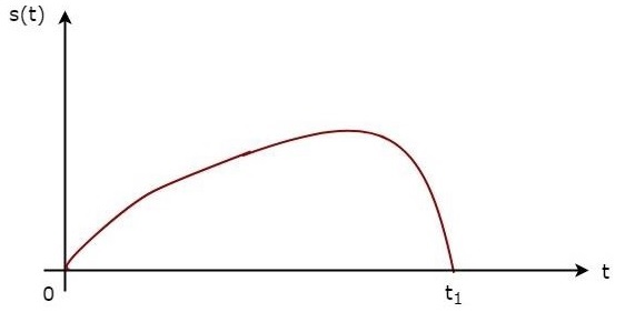
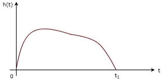
The received signal, $s\left (t\right )$ and the impulse response, $h\left (t\right )$ of the matched filter corresponding to the signal, $s\left (t\right )$ are shown in the above figures.
Radar Systems - Radar Displays
An electronic instrument, which is used for displaying the data visually is known as display. So, the electronic instrument which displays the information about Radar’s target visually is known as Radar display. It shows the echo signal information visually on the screen.
Types of Radar Displays
In this section, we will learn about the different types of Radar Displays. The Radar Displays can be classified into the following types.
A-Scope
It is a two dimensional Radar display. The horizontal and vertical coordinates represent the range and echo amplitude of the target respectively. In A-Scope, the deflection modulation takes place. It is more suitable for manually tracking Radar.
B-Scope
It is a two dimensional Radar display. The horizontal and vertical coordinates represent the azimuth angle and the range of the target respectively. In B-Scope, intensity modulation takes place. It is more suitable for military Radars.
C-Scope
It is a two-dimensional Radar display. The horizontal and vertical coordinates represent the azimuth angle and elevation angle respectively. In C-Scope, intensity modulation takes place.
D-Scope
If the electron beam is deflected or the intensity-modulated spot appears on the Radar display due to the presence of target, then it is known as blip. C-Scope becomes D-Scope, when the blips extend vertically in order to provide the distance.
E-Scope
It is a two-dimensional Radar display. The horizontal and vertical coordinates represent the distance and elevation angle respectively. In E-Scope, intensity modulation takes place.
F-Scope
If the Radar Antenna is aimed at the target, then F-Scope displays the target as a centralized blip. So, the horizontal and vertical displacements of the blip represent the horizontal and vertical aiming errors respectively.
G-Scope
If the Radar Antenna is aimed at the target, then G-Scope displays the target as laterally centralized blip. The horizontal and vertical displacements of the blip represent the horizontal and vertical aiming errors respectively.
H-Scope
It is the modified version of B-Scope in order to provide the information about elevation angle of the target. It displays the target as two blips, which are closely spaced. This can be approximated to a short bright line and the slope of this line will be proportional to the sine of the elevation angle.
I-Scope
If the Radar Antenna is aimed at the target, then I-Scope displays the target as a circle. The radius of this circle will be proportional to the distance of the target. If the Radar Antenna is aimed at the target incorrectly, then I-Scope displays the target as a segment instead of circle. The arc length of that segment will be inversely proportional to the magnitude of pointing error.
J-Scope
It is the modified version of A-Scope. It displays the target as radial deflection from time base.
K-Scope
It is the modified version of A-Scope. If the Radar Antenna is aimed at the target, then K-Scope displays the target as a pair of vertical deflections, which are having equal height. If the Radar Antenna is aimed at the target incorrectly, then there will be pointing error. So, the magnitude and the direction of the pointing error depends on the difference between the two vertical deflections.
L-Scope
If the Radar Antenna is aimed at the target, then L-Scope displays the target as two horizontal blips having equal amplitude. One horizontal blip lies to the right of central vertical time base and the other one lies to the left of central vertical time base.
M-Scope
It is the modified version of A-Scope. An adjustable pedestal signal has to be moved along the baseline till it coincides the signal deflections, which are coming from the horizontal position of the target. In this way, the target’s distance can be determined.
N-Scope
It is the modified version of K-Scope. An adjustable pedestal signal is used for measuring distance.
O-Scope
It is the modified version of A-Scope. We will get O-Scope, by including an adjustable notch to A-Scope for measuring distance.
P-Scope
It is a Radar display, which uses intensity modulation. It displays the information of echo signal as plan view. Range and azimuth angle are displayed in polar coordinates. Hence, it is called the Plan Position Indicator or the PPI display.
R-Scope
It is a Radar display, which uses intensity modulation. The horizontal and vertical coordinates represent the range and height of the target respectively. Hence, it is called Range-Height Indicator or RHI display.
Radar Systems - Duplexers
In two-way communication, if we are supposed to use the same Antenna for both transmission and reception of the signals, then we require Duplexer. Duplexer is a microwave switch, which connects the Antenna to the transmitter section for transmission of the signal. Therefore, the Radar cannot receive the signal during transmission time.
Similarly, it connects the Antenna to the receiver section for the reception of the signal. The Radar cannot transmit the signal during reception time. In this way, Duplexer isolates both transmitter and receiver sections.
Types of Duplexers
In this section, we will learn about the different types of duplexers. We can classify the Duplexers into the following three types.
- Branch-type Duplexer
- Balanced Duplexer
- Circulator as Duplexer
In our subsequent sections, we will discuss the types of Duplexers in detail.
Branch-type Duplexer
Branch-type Duplexer consists of two switches — Transmit-Receive (TR) switch and Anti Transmit-Receive (ATR) switch. The following figure shows the block diagram of Branch-type Duplexer −
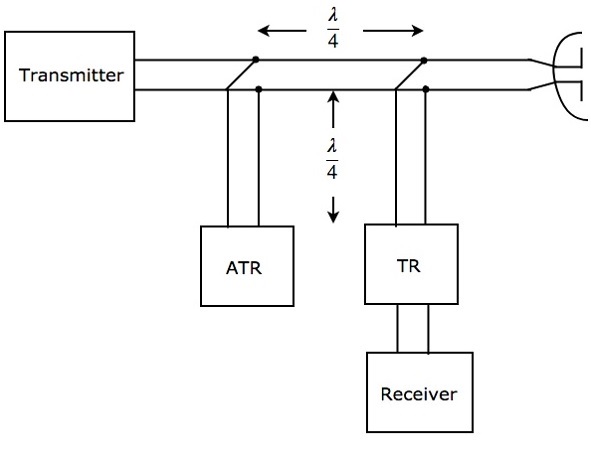
As shown in the figure, the two switches, TR & ATR are placed at a distance of $\lambda/4$ from the transmission line and both the switches are separated by a distance of $\lambda/4$. The working of Branch-type Duplexer is mentioned below.
During transmission, both TR & ATR will look like an open circuit from the transmission line. Therefore, the Antenna will be connected to the transmitter through transmission line.
During reception, ATR will look like a short circuit across the transmission line. Hence, Antenna will be connected to the receiver through transmission line.
The Branch-type Duplexer is suitable only for low cost Radars, since it is having less power handling capability.
Balanced Duplexer
We know that a two-hole Directional Coupler is a 4-port waveguide junction consisting of a primary waveguide and a secondary waveguide. There are two small holes, which will be common to those two waveguides.
The Balanced Duplexer consists of two TR tubes. The configuration of Balanced Duplexer for transmission purpose is shown in the following figure.
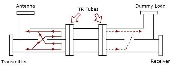
The signal, which is produced by the transmitter has to reach the Antenna for the Antenna to transmit that signal during transmission time. The solid lines with arrow marks shown in the above figure represent how the signal reaches Antenna from transmitter.
The dotted lines with arrow marks shown in the above figure represent the signal, which is leaked from the Dual TR tubes; this will reach only the matched load. So, no signal has been reached to the receiver.
The configuration of Balanced Duplexer for reception purpose is shown in figure given below.
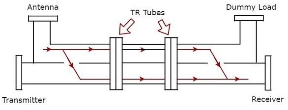
We know that Antenna receives the signal during reception time. The signal which is received by the Antenna has to reach the receiver. The solid lines with arrow marks shown in the above figure represent how the signal is reaching the receiver from Antenna. In this case, Dual TR tubes pass the signal from the first section of waveguide to the next section of waveguide.
The Balanced Duplexer has high power handling capability and high bandwidth when compared to Branch-type Duplexer.
Circulator as Duplexer
We know that the functionality of the circulator is that if we apply an input to a port, then it will be produced at the port, which is adjacent to it in the clockwise direction. There is no output at the remaining ports of the circulator.
So, consider a 4-port circulator and connect the transmitter, Antenna, receiver and matched load to port1, port2, port3 and port4 respectively. Now, let us understand how the 4-port circulator works as Duplexer.
The signal, which is produced by the transmitter has to reach the Antenna for the Antenna will transmit that signal during transmission time. This purpose will be achieved when the transmitter generates a signal at port1.
The signal, which is received by the Antenna has to reach the receiver during reception time. This purpose will be achieved when the Antenna present at port2 receives an external signal.
The following figure shows the block diagram of circulator as Duplexer −
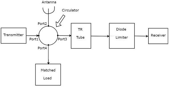
The above figure consists of a 4-port circulator — Transmitter, Antenna and the matched load is connected to port1, port2 and port4 of circulator respectively as discussed in the beginning of the section.
The receiver is not directly connected to port3. Instead, the blocks corresponding to the passive TR limiter are placed between port3 of circulator and receiver. The blocks, TR tube & Diode limiter are the blocks corresponding to passive TR limiter.
Actually, the circulator itself acts as Duplexer. It does not require any additional blocks. However, it will not give any kind of protection to the receiver. Hence, the blocks corresponding to passive TR limiter are used in order to provide the protection to the receiver.
Radar Systems - Phased Array Antennas
A single Antenna can radiate certain amount of power in a particular direction. Obviously, the amount of radiation power will be increased when we use group of Antennas together. The group of Antennas is called Antenna array.
An Antenna array is a radiating system comprising radiators and elements. Each of this radiator has its own induction field. The elements are placed so closely that each one lies in the neighbouring one’s induction field. Therefore, the radiation pattern produced by them, would be the vector sum of the individual ones.
The Antennas radiate individually and while in an array, the radiation of all the elements sum up, to form the radiation beam, which has high gain, high directivity and better performance, with minimum losses.
An Antenna array is said to be Phased Antenna array if the shape and direction of the radiation pattern depends on the relative phases and amplitudes of the currents present at each Antenna of that array.
Radiation Pattern
Let us consider ‘n’ isotropic radiation elements, which when combined form an array. The figure given below will help you understand the same. Let the spacing between the successive elements be ‘d’ units.
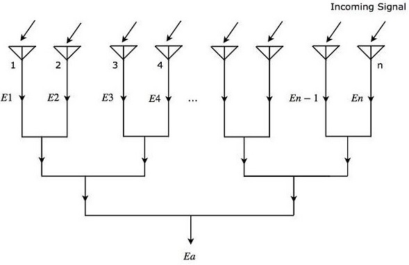
As shown in the figure, all the radiation elements receive the same incoming signal. So, each element produces an equal output voltage of $sin \left ( \omega t \right)$. However, there will be an equal phase difference $\Psi$ between successive elements. Mathematically, it can be written as −
$$\Psi=\frac{2\pi d\sin\theta }{\lambda }\:\:\:\:\:Equation\:1$$
Where,
$\theta$ is the angle at which the incoming signal is incident on each radiation element.
Mathematically, we can write the expressions for output voltages of ‘n’ radiation elements individually as
$$E_1=\sin\left [ \omega t \right]$$
$$E_2=\sin\left [\omega t+\Psi\right]$$
$$E_3=\sin\left [\omega t+2\Psi\right]$$
$$.$$
$$.$$
$$.$$
$$E_n=\sin\left [\omega t+\left (N-1\right )\Psi\right]$$
Where,
$E_1, E_2, E_3, …, E_n$ are the output voltages of first, second, third, …, nth radiation elements respectively.
$\omega$ is the angular frequency of the signal.
We will get the overall output voltage $E_a$ of the array by adding the output voltages of each element present in that array, since all those radiation elements are connected in linear array. Mathematically, it can be represented as −
$$E_a=E_1+E_2+E_3+ …+E_n \:\:\:Equation\:2$$
Substitute, the values of $E_1, E_2, E_3, …, E_n$ in Equation 2.
$$E_a=\sin\left [ \omega t \right]+\sin\left [\omega t+\Psi\right ]+\sin\left [\omega t+2\Psi\right ]+\sin\left [\omega t+\left (n-1\right )\Psi\right]$$
$$\Rightarrow E_a=\sin\left [\omega t+\frac{(n-1)\Psi)}{2}\right ]\frac{\sin\left [\frac{n\Psi}{2}\right]}{\sin\left [\frac{\Psi}{2}\right ]}\:\:\:\:\:Equation\:3$$
In Equation 3, there are two terms. From first term, we can observe that the overall output voltage $E_a$ is a sine wave having an angular frequency $\omega$. But, it is having a phase shift of $\left (n−1\right )\Psi/2$. The second term of Equation 3 is an amplitude factor.
The magnitude of Equation 3 will be
$$\left | E_a \right|=\left | \frac{\sin\left [\frac{n\Psi}{2}\right ]}{\sin\left [\frac{\Psi}{2}\right]} \right |\:\:\:\:\:Equation\:4$$
We will get the following equation by substituting Equation 1 in Equation 4.
$$\left | E_a \right|=\left | \frac{\sin\left [\frac{n\pi d\sin\theta}{\lambda}\right]}{\sin\left [\frac{\pi d\sin\theta}{\lambda}\right ]} \right |\:\:\:\:\:Equation\:5$$
Equation 5 is called field intensity pattern. The field intensity pattern will have the values of zeros when the numerator of Equation 5 is zero
$$\sin\left [\frac{n\pi d\sin\theta}{\lambda}\right ]=0$$
$$\Rightarrow \frac{n\pi d\sin\theta}{\lambda}=\pm m\pi$$
$$\Rightarrow nd\sin\theta=\pm m\lambda$$
$$\Rightarrow \sin\theta=\pm \frac{m\lambda}{nd}$$
Where,
$m$ is an integer and it is equal to 1, 2, 3 and so on.
We can find the maximum values of field intensity pattern by using L-Hospital rule when both numerator and denominator of Equation 5 are equal to zero. We can observe that if the denominator of Equation 5 becomes zero, then the numerator of Equation 5 also becomes zero.
Now, let us get the condition for which the denominator of Equation 5 becomes zero.
$$\sin\left [\frac{\pi d\sin\theta}{\lambda}\right ]=0$$
$$\Rightarrow \frac{\pi d\sin\theta}{\lambda}=\pm p\pi$$
$$\Rightarrow d\sin\theta=\pm p\lambda$$
$$\Rightarrow \sin\theta=\pm \frac{p\lambda}{d}$$
Where,
$p$ is an integer and it is equal to 0, 1, 2, 3 and so on.
If we consider $p$ as zero, then we will get the value of $\sin\theta$ as zero. For this case, we will get the maximum value of field intensity pattern corresponding to the main lobe. We will get the maximum values of field intensity pattern corresponding to side lobes, when we consider other values of $p$.
The radiation pattern’s direction of phased array can be steered by varying the relative phases of the current present at each Antenna. This is the advantage of electronic scanning phased array.