- PyTorch Tutorial
- PyTorch - Home
- PyTorch - Introduction
- PyTorch - Installation
- Mathematical Building Blocks of Neural Networks
- PyTorch - Neural Network Basics
- Universal Workflow of Machine Learning
- Machine Learning vs. Deep Learning
- Implementing First Neural Network
- Neural Networks to Functional Blocks
- PyTorch - Terminologies
- PyTorch - Loading Data
- PyTorch - Linear Regression
- PyTorch - Convolutional Neural Network
- PyTorch - Recurrent Neural Network
- PyTorch - Datasets
- PyTorch - Introduction to Convents
- Training a Convent from Scratch
- PyTorch - Feature Extraction in Convents
- PyTorch - Visualization of Convents
- Sequence Processing with Convents
- PyTorch - Word Embedding
- PyTorch - Recursive Neural Networks
- PyTorch Useful Resources
- PyTorch - Quick Guide
- PyTorch - Useful Resources
- PyTorch - Discussion
PyTorch - Quick Guide
PyTorch - Introduction
PyTorch is defined as an open source machine learning library for Python. It is used for applications such as natural language processing. It is initially developed by Facebook artificial-intelligence research group, and Uber’s Pyro software for probabilistic programming which is built on it.
Originally, PyTorch was developed by Hugh Perkins as a Python wrapper for the LusJIT based on Torch framework. There are two PyTorch variants.
PyTorch redesigns and implements Torch in Python while sharing the same core C libraries for the backend code. PyTorch developers tuned this back-end code to run Python efficiently. They also kept the GPU based hardware acceleration as well as the extensibility features that made Lua-based Torch.
Features
The major features of PyTorch are mentioned below −
Easy Interface − PyTorch offers easy to use API; hence it is considered to be very simple to operate and runs on Python. The code execution in this framework is quite easy.
Python usage − This library is considered to be Pythonic which smoothly integrates with the Python data science stack. Thus, it can leverage all the services and functionalities offered by the Python environment.
Computational graphs − PyTorch provides an excellent platform which offers dynamic computational graphs. Thus a user can change them during runtime. This is highly useful when a developer has no idea of how much memory is required for creating a neural network model.
PyTorch is known for having three levels of abstraction as given below −
Tensor − Imperative n-dimensional array which runs on GPU.
Variable − Node in computational graph. This stores data and gradient.
Module − Neural network layer which will store state or learnable weights.
Advantages of PyTorch
The following are the advantages of PyTorch −
It is easy to debug and understand the code.
It includes many layers as Torch.
It includes lot of loss functions.
It can be considered as NumPy extension to GPUs.
It allows building networks whose structure is dependent on computation itself.
TensorFlow vs. PyTorch
We shall look into the major differences between TensorFlow and PyTorch below −
| PyTorch | TensorFlow |
|---|---|
PyTorch is closely related to the lua-based Torch framework which is actively used in Facebook. |
TensorFlow is developed by Google Brain and actively used at Google. |
PyTorch is relatively new compared to other competitive technologies. |
TensorFlow is not new and is considered as a to-go tool by many researchers and industry professionals. |
PyTorch includes everything in imperative and dynamic manner. |
TensorFlow includes static and dynamic graphs as a combination. |
Computation graph in PyTorch is defined during runtime. |
TensorFlow do not include any run time option. |
PyTorch includes deployment featured for mobile and embedded frameworks. |
TensorFlow works better for embedded frameworks. |
PyTorch - Installation
PyTorch is a popular deep learning framework. In this tutorial, we consider “Windows 10” as our operating system. The steps for a successful environmental setup are as follows −
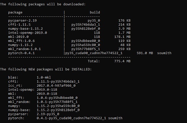
Step 1
The following link includes a list of packages which includes suitable packages for PyTorch.
https://drive.google.com/drive/folders/0B-X0-FlSGfCYdTNldW02UGl4MXMAll you need to do is download the respective packages and install it as shown in the following screenshots −
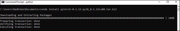
Step 2
It involves verifying the installation of PyTorch framework using Anaconda Framework.
Following command is used to verify the same −
conda list
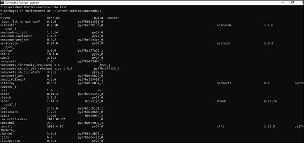
“Conda list” shows the list of frameworks which is installed.
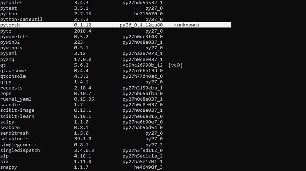
The highlighted part shows that PyTorch has been successfully installed in our system.
Mathematical Building Blocks of Neural Networks
Mathematics is vital in any machine learning algorithm and includes various core concepts of mathematics to get the right algorithm designed in a specific way.
The importance of mathematics topics for machine learning and data science is mentioned below −
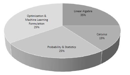
Now, let us focus on the major mathematical concepts of machine learning which is important from Natural Language Processing point of view −
Vectors
Vector is considered to be array of numbers which is either continuous or discrete and the space which consists of vectors is called as vector space. The space dimensions of vectors can be either finite or infinite but it has been observed that machine learning and data science problems deal with fixed length vectors.
The vector representation is displayed as mentioned below −
temp = torch.FloatTensor([23,24,24.5,26,27.2,23.0])
temp.size()
Output - torch.Size([6])
In machine learning, we deal with multidimensional data. So vectors become very crucial and are considered as input features for any prediction problem statement.
Scalars
Scalars are termed to have zero dimensions containing only one value. When it comes to PyTorch, it does not include a special tensor with zero dimensions; hence the declaration will be made as follows −
x = torch.rand(10)
x.size()
Output - torch.Size([10])
Matrices
Most of the structured data is usually represented in the form of tables or a specific matrix. We will use a dataset called Boston House Prices, which is readily available in the Python scikit-learn machine learning library.
boston_tensor = torch.from_numpy(boston.data)
boston_tensor.size()
Output: torch.Size([506, 13])
boston_tensor[:2]
Output:
Columns 0 to 7
0.0063 18.0000 2.3100 0.0000 0.5380 6.5750 65.2000 4.0900
0.0273 0.0000 7.0700 0.0000 0.4690 6.4210 78.9000 4.9671
Columns 8 to 12
1.0000 296.0000 15.3000 396.9000 4.9800
2.0000 242.0000 17.8000 396.9000 9.1400
PyTorch - Neural Network Basics
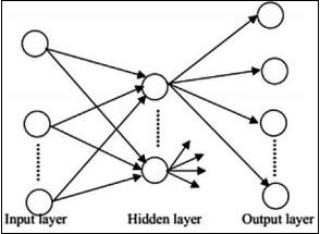
The main principle of neural network includes a collection of basic elements, i.e., artificial neuron or perceptron. It includes several basic inputs such as x1, x2….. xn which produces a binary output if the sum is greater than the activation potential.
The schematic representation of sample neuron is mentioned below −
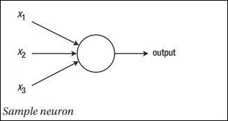
The output generated can be considered as the weighted sum with activation potential or bias.
$$Output=\sum_jw_jx_j+Bias$$
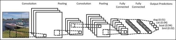
The typical neural network architecture is described below −
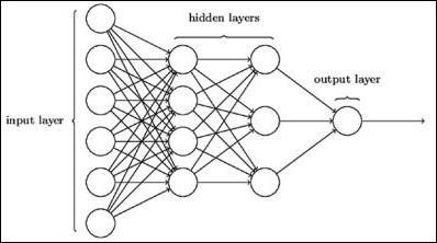
The layers between input and output are referred to as hidden layers, and the density and type of connections between layers is the configuration. For example, a fully connected configuration has all the neurons of layer L connected to those of L+1. For a more pronounced localization, we can connect only a local neighbourhood, say nine neurons, to the next layer. Figure 1-9 illustrates two hidden layers with dense connections.
The various types of neural networks are as follows −
Feedforward Neural Networks
Feedforward neural networks include basic units of neural network family. The movement of data in this type of neural network is from the input layer to output layer, via present hidden layers. The output of one layer serves as the input layer with restrictions on any kind of loops in the network architecture.
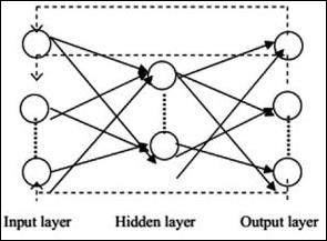
Recurrent Neural Networks
Recurrent Neural Networks are when the data pattern changes consequently over a period. In RNN, same layer is applied to accept the input parameters and display output parameters in specified neural network.
Neural networks can be constructed using the torch.nn package.
It is a simple feed-forward network. It takes the input, feeds it through several layers one after the other, and then finally gives the output.
With the help of PyTorch, we can use the following steps for typical training procedure for a neural network −
- Define the neural network that has some learnable parameters (or weights).
- Iterate over a dataset of inputs.
- Process input through the network.
- Compute the loss (how far is the output from being correct).
- Propagate gradients back into the network’s parameters.
- Update the weights of the network, typically using a simple update as given below
rule: weight = weight -learning_rate * gradient
Universal Workflow of Machine Learning
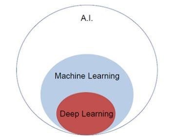
Artificial Intelligence is trending nowadays to a greater extent. Machine learning and deep learning constitutes artificial intelligence. The Venn diagram mentioned below explains the relationship of machine learning and deep learning.
Machine Learning
Machine learning is the art of science which allows computers to act as per the designed and programmed algorithms. Many researchers think machine learning is the best way to make progress towards human-level AI. It includes various types of patterns like −
- Supervised Learning Pattern
- Unsupervised Learning Pattern
Deep Learning
Deep learning is a subfield of machine learning where concerned algorithms are inspired by the structure and function of the brain called Artificial Neural Networks.
Deep learning has gained much importance through supervised learning or learning from labelled data and algorithms. Each algorithm in deep learning goes through same process. It includes hierarchy of nonlinear transformation of input and uses to create a statistical model as output.
Machine learning process is defined using following steps −
- Identifies relevant data sets and prepares them for analysis.
- Chooses the type of algorithm to use.
- Builds an analytical model based on the algorithm used.
- Trains the model on test data sets, revising it as needed.
- Runs the model to generate test scores.
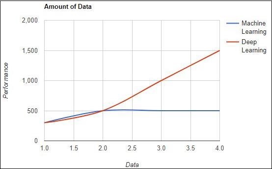
PyTorch - Machine Learning vs. Deep Learning
In this chapter, we will discuss the major difference between Machine and Deep learning concepts.
Amount of Data
Machine learning works with different amounts of data and is mainly used for small amounts of data. Deep learning on the other hand works efficiently if the amount of data increases rapidly. The following diagram depicts the working of machine learning and deep learning with respect to amount of data −
Hardware Dependencies
Deep learning algorithms are designed to heavily depend on high end machines on a contrary to traditional machine learning algorithms. Deep learning algorithms perform a large amount of matrix multiplication operations which requires a huge hardware support.
Feature Engineering
Feature engineering is the process of putting domain knowledge into specified features to reduce the complexity of data and make patterns which are visible to learning algorithms.
For instance, traditional machine learning patterns focusses on pixels and other attributes needed for feature engineering process. Deep learning algorithms focusses on high level features from data. It reduces the task of developing new feature extractor for every new problem.
PyTorch - Implementing First Neural Network
PyTorch includes a special feature of creating and implementing neural networks. In this chapter, we will create a simple neural network with one hidden layer developing a single output unit.
We shall use following steps to implement the first neural network using PyTorch −
Step 1
First, we need to import the PyTorch library using the below command −
import torch
import torch.nn as nn
Step 2
Define all the layers and the batch size to start executing the neural network as shown below −
# Defining input size, hidden layer size, output size and batch size respectively
n_in, n_h, n_out, batch_size = 10, 5, 1, 10
Step 3
As neural network includes a combination of input data to get the respective output data, we will be following the same procedure as given below −
# Create dummy input and target tensors (data)
x = torch.randn(batch_size, n_in)
y = torch.tensor([[1.0], [0.0], [0.0],
[1.0], [1.0], [1.0], [0.0], [0.0], [1.0], [1.0]])
Step 4
Create a sequential model with the help of in-built functions. Using the below lines of code, create a sequential model −
# Create a model
model = nn.Sequential(nn.Linear(n_in, n_h),
   nn.ReLU(),
   nn.Linear(n_h, n_out),
   nn.Sigmoid())
Step 5
Construct the loss function with the help of Gradient Descent optimizer as shown below −
Construct the loss function
criterion = torch.nn.MSELoss()
# Construct the optimizer (Stochastic Gradient Descent in this case)
optimizer = torch.optim.SGD(model.parameters(), lr = 0.01)
Step 6
Implement the gradient descent model with the iterating loop with the given lines of code −
# Gradient Descent
for epoch in range(50):
   # Forward pass: Compute predicted y by passing x to the model
   y_pred = model(x)

   # Compute and print loss
   loss = criterion(y_pred, y)
   print('epoch: ', epoch,' loss: ', loss.item())

   # Zero gradients, perform a backward pass, and update the weights.
   optimizer.zero_grad()

   # perform a backward pass (backpropagation)
   loss.backward()

   # Update the parameters
   optimizer.step()
Step 7
The output generated is as follows −
epoch: 0 loss: 0.2545787990093231
epoch: 1 loss: 0.2545052170753479
epoch: 2 loss: 0.254431813955307
epoch: 3 loss: 0.25435858964920044
epoch: 4 loss: 0.2542854845523834
epoch: 5 loss: 0.25421255826950073
epoch: 6 loss: 0.25413978099823
epoch: 7 loss: 0.25406715273857117
epoch: 8 loss: 0.2539947032928467
epoch: 9 loss: 0.25392240285873413
epoch: 10 loss: 0.25385022163391113
epoch: 11 loss: 0.25377824902534485
epoch: 12 loss: 0.2537063956260681
epoch: 13 loss: 0.2536346912384033
epoch: 14 loss: 0.25356316566467285
epoch: 15 loss: 0.25349172949790955
epoch: 16 loss: 0.25342053174972534
epoch: 17 loss: 0.2533493936061859
epoch: 18 loss: 0.2532784342765808
epoch: 19 loss: 0.25320762395858765
epoch: 20 loss: 0.2531369626522064
epoch: 21 loss: 0.25306645035743713
epoch: 22 loss: 0.252996027469635
epoch: 23 loss: 0.2529257833957672
epoch: 24 loss: 0.25285571813583374
epoch: 25 loss: 0.25278574228286743
epoch: 26 loss: 0.25271597504615784
epoch: 27 loss: 0.25264623761177063
epoch: 28 loss: 0.25257670879364014
epoch: 29 loss: 0.2525072991847992
epoch: 30 loss: 0.2524380087852478
epoch: 31 loss: 0.2523689270019531
epoch: 32 loss: 0.25229987502098083
epoch: 33 loss: 0.25223103165626526
epoch: 34 loss: 0.25216227769851685
epoch: 35 loss: 0.252093642950058
epoch: 36 loss: 0.25202515721321106
epoch: 37 loss: 0.2519568204879761
epoch: 38 loss: 0.251888632774353
epoch: 39 loss: 0.25182053446769714
epoch: 40 loss: 0.2517525553703308
epoch: 41 loss: 0.2516847252845764
epoch: 42 loss: 0.2516169846057892
epoch: 43 loss: 0.2515493929386139
epoch: 44 loss: 0.25148195028305054
epoch: 45 loss: 0.25141456723213196
epoch: 46 loss: 0.2513473629951477
epoch: 47 loss: 0.2512802183628082
epoch: 48 loss: 0.2512132525444031
epoch: 49 loss: 0.2511464059352875
PyTorch - Neural Networks to Functional Blocks
Training a deep learning algorithm involves the following steps −
- Building a data pipeline
- Building a network architecture
- Evaluating the architecture using a loss function
- Optimizing the network architecture weights using an optimization algorithm
Training a specific deep learning algorithm is the exact requirement of converting a neural network to functional blocks as shown below −
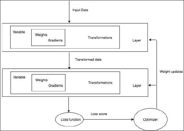
With respect to the above diagram, any deep learning algorithm involves getting the input data, building the respective architecture which includes a bunch of layers embedded in them.
If you observe the above diagram, the accuracy is evaluated using a loss function with respect to optimization of the weights of neural network.
PyTorch - Terminologies
In this chapter, we will discuss some of the most commonly used terms in PyTorch.
PyTorch NumPy
A PyTorch tensor is identical to a NumPy array. A tensor is an n-dimensional array and with respect to PyTorch, it provides many functions to operate on these tensors.
PyTorch tensors usually utilize GPUs to accelerate their numeric computations. These tensors which are created in PyTorch can be used to fit a two-layer network to random data. The user can manually implement the forward and backward passes through the network.
Variables and Autograd
When using autograd, the forward pass of your network will define a computational graph − nodes in the graph will be Tensors, and edges will be functions that produce output Tensors from input Tensors.
PyTorch Tensors can be created as variable objects where a variable represents a node in computational graph.
Dynamic Graphs
Static graphs are nice because user can optimize the graph up front. If programmers are re-using same graph over and over, then this potentially costly up-front optimization can be maintained as the same graph is rerun over and over.
The major difference between them is that Tensor Flow’s computational graphs are static and PyTorch uses dynamic computational graphs.
Optim Package
The optim package in PyTorch abstracts the idea of an optimization algorithm which is implemented in many ways and provides illustrations of commonly used optimization algorithms. This can be called within the import statement.
Multiprocessing
Multiprocessing supports the same operations, so that all tensors work on multiple processors. The queue will have their data moved into shared memory and will only send a handle to another process.
PyTorch - Loading Data
PyTorch includes a package called torchvision which is used to load and prepare the dataset. It includes two basic functions namely Dataset and DataLoader which helps in transformation and loading of dataset.
Dataset
Dataset is used to read and transform a datapoint from the given dataset. The basic syntax to implement is mentioned below −
trainset = torchvision.datasets.CIFAR10(root = './data', train = True,
   download = True, transform = transform)
DataLoader is used to shuffle and batch data. It can be used to load the data in parallel with multiprocessing workers.
trainloader = torch.utils.data.DataLoader(trainset, batch_size = 4,
   shuffle = True, num_workers = 2)
Example: Loading CSV File
We use the Python package Panda to load the csv file. The original file has the following format: (image name, 68 landmarks - each landmark has a x, y coordinates).
landmarks_frame = pd.read_csv('faces/face_landmarks.csv')

n = 65
img_name = landmarks_frame.iloc[n, 0]
landmarks = landmarks_frame.iloc[n, 1:].as_matrix()
landmarks = landmarks.astype('float').reshape(-1, 2)
PyTorch - Linear Regression
In this chapter, we will be focusing on basic example of linear regression implementation using TensorFlow. Logistic regression or linear regression is a supervised machine learning approach for the classification of order discrete categories. Our goal in this chapter is to build a model by which a user can predict the relationship between predictor variables and one or more independent variables.
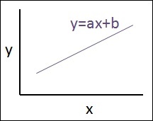
The relationship between these two variables is considered linear i.e., if y is the dependent variable and x is considered as the independent variable, then the linear regression relationship of two variables will look like the equation which is mentioned as below −
Y = Ax+b
Next, we shall design an algorithm for linear regression which allows us to understand two important concepts given below −
- Cost Function
- Gradient Descent Algorithms
The schematic representation of linear regression is mentioned below
Interpreting the result
$$Y=ax+b$$
The value of a is the slope.
The value of b is the y − intercept.
r is the correlation coefficient.
r2 is the correlation coefficient.
The graphical view of the equation of linear regression is mentioned below −
Following steps are used for implementing linear regression using PyTorch −
Step 1
Import the necessary packages for creating a linear regression in PyTorch using the below code −
import numpy as np
import matplotlib.pyplot as plt
from matplotlib.animation import FuncAnimation
import seaborn as sns
import pandas as pd
%matplotlib inline

sns.set_style(style = 'whitegrid')
plt.rcParams["patch.force_edgecolor"] = True
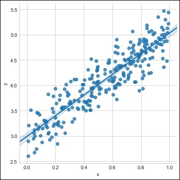
Step 2
Create a single training set with the available data set as shown below −
m = 2 # slope
c = 3 # interceptm = 2 # slope
c = 3 # intercept
x = np.random.rand(256)

noise = np.random.randn(256) / 4

y = x * m + c + noise

df = pd.DataFrame()
df['x'] = x
df['y'] = y

sns.lmplot(x ='x', y ='y', data = df)
Step 3
Implement linear regression with PyTorch libraries as mentioned below −
import torch
import torch.nn as nn
from torch.autograd import Variable
x_train = x.reshape(-1, 1).astype('float32')
y_train = y.reshape(-1, 1).astype('float32')
class LinearRegressionModel(nn.Module):
def __init__(self, input_dim, output_dim):
super(LinearRegressionModel, self).__init__()
self.linear = nn.Linear(input_dim, output_dim)
def forward(self, x):
out = self.linear(x)
return out
input_dim = x_train.shape[1]
output_dim = y_train.shape[1]
input_dim, output_dim(1, 1)
model = LinearRegressionModel(input_dim, output_dim)
criterion = nn.MSELoss()
[w, b] = model.parameters()
def get_param_values():
return w.data[0][0], b.data[0]
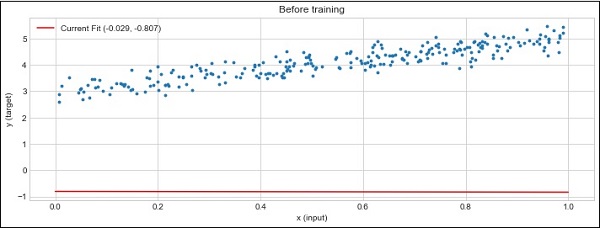
def plot_current_fit(title = ""):
plt.figure(figsize = (12,4))
plt.title(title)
plt.scatter(x, y, s = 8)
w1 = w.data[0][0]
b1 = b.data[0]
x1 = np.array([0., 1.])
y1 = x1 * w1 + b1
plt.plot(x1, y1, 'r', label = 'Current Fit ({:.3f}, {:.3f})'.format(w1, b1))
plt.xlabel('x (input)')
plt.ylabel('y (target)')
plt.legend()
plt.show()
plot_current_fit('Before training')
The plot generated is as follows −
PyTorch - Convolutional Neural Network
Deep learning is a division of machine learning and is considered as a crucial step taken by researchers in recent decades. The examples of deep learning implementation include applications like image recognition and speech recognition.
The two important types of deep neural networks are given below −
- Convolutional Neural Networks
- Recurrent Neural Networks.
In this chapter, we will be focusing on the first type, i.e., Convolutional Neural Networks (CNN).
Convolutional Neural Networks
Convolutional Neural networks are designed to process data through multiple layers of arrays. This type of neural networks are used in applications like image recognition or face recognition.
The primary difference between CNN and any other ordinary neural network is that CNN takes input as a two dimensional array and operates directly on the images rather than focusing on feature extraction which other neural networks focus on.
The dominant approach of CNN includes solution for problems of recognition. Top companies like Google and Facebook have invested in research and development projects of recognition projects to get activities done with greater speed.
Every convolutional neural network includes three basic ideas −
- Local respective fields
- Convolution
- Pooling
Let us understand each of these terminologies in detail.
Local Respective Fields
CNN utilize spatial correlations that exists within the input data. Each in the concurrent layers of neural networks connects of some input neurons. This specific region is called Local Receptive Field. It only focusses on hidden neurons. The hidden neuron will process the input data inside the mentioned field not realizing the changes outside the specific boundary.
The diagram representation of generating local respective fields is mentioned below −
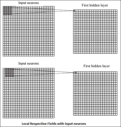
Convolution
In the above figure, we observe that each connection learns a weight of hidden neuron with an associated connection with movement from one layer to another. Here, individual neurons perform a shift from time to time. This process is called “convolution”.
The mapping of connections from the input layer to the hidden feature map is defined as “shared weights” and bias included is called “shared bias”.
Pooling
Convolutional neural networks use pooling layers which are positioned immediately after CNN declaration. It takes the input from the user as a feature map which comes out convolutional networks and prepares a condensed feature map. Pooling layers help in creating layers with neurons of previous layers.
Implementation of PyTorch
Following steps are used to create a Convolutional Neural Network using PyTorch.
Step 1
Import the necessary packages for creating a simple neural network.
from torch.autograd import Variable
import torch.nn.functional as F
Step 2
Create a class with batch representation of convolutional neural network. Our batch shape for input x is with dimension of (3, 32, 32).
class SimpleCNN(torch.nn.Module):
   def __init__(self):
      super(SimpleCNN, self).__init__()
      #Input channels = 3, output channels = 18
      self.conv1 = torch.nn.Conv2d(3, 18, kernel_size = 3, stride = 1, padding = 1)
      self.pool = torch.nn.MaxPool2d(kernel_size = 2, stride = 2, padding = 0)
      #4608 input features, 64 output features (see sizing flow below)
      self.fc1 = torch.nn.Linear(18 * 16 * 16, 64)
      #64 input features, 10 output features for our 10 defined classes
      self.fc2 = torch.nn.Linear(64, 10)
Step 3
Compute the activation of the first convolution size changes from (3, 32, 32) to (18, 32, 32).
Size of the dimension changes from (18, 32, 32) to (18, 16, 16). Reshape data dimension of the input layer of the neural net due to which size changes from (18, 16, 16) to (1, 4608).
Recall that -1 infers this dimension from the other given dimension.
def forward(self, x):
   x = F.relu(self.conv1(x))
   x = self.pool(x)
   x = x.view(-1, 18 * 16 *16)
   x = F.relu(self.fc1(x))
   #Computes the second fully connected layer (activation applied later)
   #Size changes from (1, 64) to (1, 10)
   x = self.fc2(x)
   return(x)
PyTorch - Recurrent Neural Network
Recurrent neural networks is one type of deep learning-oriented algorithm which follows a sequential approach. In neural networks, we always assume that each input and output is independent of all other layers. These type of neural networks are called recurrent because they perform mathematical computations in a sequential manner completing one task after another.
The diagram below specifies the complete approach and working of recurrent neural networks −
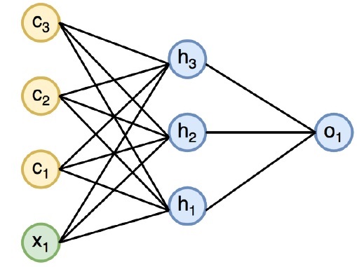
In the above figure, c1, c2, c3 and x1 are considered as inputs which includes some hidden input values namely h1, h2 and h3 delivering the respective output of o1. We will now focus on implementing PyTorch to create a sine wave with the help of recurrent neural networks.
During training, we will follow a training approach to our model with one data point at a time. The input sequence x consists of 20 data points, and the target sequence is considered to be same as the input sequence.
Step 1
Import the necessary packages for implementing recurrent neural networks using the below code −
import torch
from torch.autograd import Variable
import numpy as np
import pylab as pl
import torch.nn.init as init
Step 2
We will set the model hyper parameters with the size of input layer set to 7. There will be 6 context neurons and 1 input neuron for creating target sequence.
dtype = torch.FloatTensor
input_size, hidden_size, output_size = 7, 6, 1
epochs = 300
seq_length = 20
lr = 0.1
data_time_steps = np.linspace(2, 10, seq_length + 1)
data = np.sin(data_time_steps)
data.resize((seq_length + 1, 1))

x = Variable(torch.Tensor(data[:-1]).type(dtype), requires_grad=False)
y = Variable(torch.Tensor(data[1:]).type(dtype), requires_grad=False)
We will generate training data, where x is the input data sequence and y is required target sequence.
Step 3
Weights are initialized in the recurrent neural network using normal distribution with zero mean. W1 will represent acceptance of input variables and w2 will represent the output which is generated as shown below −
w1 = torch.FloatTensor(input_size,
hidden_size).type(dtype)
init.normal(w1, 0.0, 0.4)
w1 = Variable(w1, requires_grad = True)
w2 = torch.FloatTensor(hidden_size, output_size).type(dtype)
init.normal(w2, 0.0, 0.3)
w2 = Variable(w2, requires_grad = True)
Step 4
Now, it is important to create a function for feed forward which uniquely defines the neural network.
def forward(input, context_state, w1, w2):
   xh = torch.cat((input, context_state), 1)
   context_state = torch.tanh(xh.mm(w1))
   out = context_state.mm(w2)
   return (out, context_state)
Step 5
The next step is to start training procedure of recurrent neural network’s sine wave implementation. The outer loop iterates over each loop and the inner loop iterates through the element of sequence. Here, we will also compute Mean Square Error (MSE) which helps in the prediction of continuous variables.
for i in range(epochs):
   total_loss = 0
   context_state = Variable(torch.zeros((1, hidden_size)).type(dtype), requires_grad = True)
   for j in range(x.size(0)):
      input = x[j:(j+1)]
      target = y[j:(j+1)]
      (pred, context_state) = forward(input, context_state, w1, w2)
      loss = (pred - target).pow(2).sum()/2
      total_loss += loss
      loss.backward()
      w1.data -= lr * w1.grad.data
      w2.data -= lr * w2.grad.data
      w1.grad.data.zero_()
      w2.grad.data.zero_()
      context_state = Variable(context_state.data)
   if i % 10 == 0:
      print("Epoch: {} loss {}".format(i, total_loss.data[0]))

context_state = Variable(torch.zeros((1, hidden_size)).type(dtype), requires_grad = False)
predictions = []

for i in range(x.size(0)):
   input = x[i:i+1]
   (pred, context_state) = forward(input, context_state, w1, w2)
   context_state = context_state
   predictions.append(pred.data.numpy().ravel()[0])
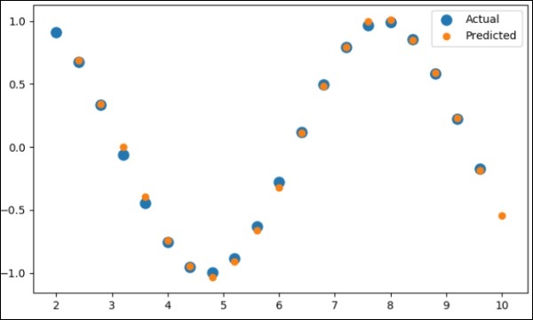
Step 6
Now, it is time to plot the sine wave as the way it is needed.
pl.scatter(data_time_steps[:-1], x.data.numpy(), s = 90, label = "Actual")
pl.scatter(data_time_steps[1:], predictions, label = "Predicted")
pl.legend()
pl.show()
Output
The output for the above process is as follows −
PyTorch - Datasets
In this chapter, we will focus more on torchvision.datasets and its various types. PyTorch includes following dataset loaders −
- MNIST
- COCO (Captioning and Detection)
Dataset includes majority of two types of functions given below −
Transform − a function that takes in an image and returns a modified version of standard stuff. These can be composed together with transforms.
Target_transform − a function that takes the target and transforms it. For example, takes in the caption string and returns a tensor of world indices.
MNIST
The following is the sample code for MNIST dataset −
dset.MNIST(root, train = TRUE, transform = NONE,
target_transform = None, download = FALSE)
The parameters are as follows −
root − root directory of the dataset where processed data exist.
train − True = Training set, False = Test set
download − True = downloads the dataset from the internet and puts it in the root.
COCO
This requires the COCO API to be installed. The following example is used to demonstrate the COCO implementation of dataset using PyTorch −
import torchvision.dataset as dset
import torchvision.transforms as transforms
cap = dset.CocoCaptions(root = ‘ dir where images are’,
annFile = ’json annotation file’,
transform = transforms.ToTensor())
print(‘Number of samples: ‘, len(cap))
print(target)
The output achieved is as follows −
Number of samples: 82783
Image Size: (3L, 427L, 640L)
PyTorch - Introduction to Convents
Convents is all about building the CNN model from scratch. The network architecture will contain a combination of following steps −
- Conv2d
- MaxPool2d
- Rectified Linear Unit
- View
- Linear Layer
Training the Model
Training the model is the same process like image classification problems. The following code snippet completes the procedure of a training model on the provided dataset −
def fit(epoch,model,data_loader,phase
= 'training',volatile = False):
   if phase == 'training':
      model.train()
   if phase == 'training':
      model.train()
   if phase == 'validation':
      model.eval()
   volatile=True
   running_loss = 0.0
   running_correct = 0
   for batch_idx , (data,target) in enumerate(data_loader):
      if is_cuda:
         data,target = data.cuda(),target.cuda()
         data , target = Variable(data,volatile),Variable(target)
      if phase == 'training':
         optimizer.zero_grad()
         output = model(data)
         loss = F.nll_loss(output,target)
         running_loss + =
         F.nll_loss(output,target,size_average =
         False).data[0]
         preds = output.data.max(dim = 1,keepdim = True)[1]
         running_correct + =
         preds.eq(target.data.view_as(preds)).cpu().sum()
         if phase == 'training':
            loss.backward()
            optimizer.step()
   loss = running_loss/len(data_loader.dataset)
   accuracy = 100. * running_correct/len(data_loader.dataset)
   print(f'{phase} loss is {loss:{5}.{2}} and {phase} accuracy is {running_correct}/{len(data_loader.dataset)}{accuracy:{return loss,accuracy}})
The method includes different logic for training and validation. There are two primary reasons for using different modes −
In train mode, dropout removes a percentage of values, which should not happen in the validation or testing phase.
For training mode, we calculate gradients and change the model's parameters value, but back propagation is not required during the testing or validation phases.
PyTorch - Training a Convent from Scratch
In this chapter, we will focus on creating a convent from scratch. This infers in creating the respective convent or sample neural network with torch.
Step 1
Create a necessary class with respective parameters. The parameters include weights with random value.
class Neural_Network(nn.Module):
   def __init__(self, ):
      super(Neural_Network, self).__init__()
      self.inputSize = 2
      self.outputSize = 1
      self.hiddenSize = 3
      # weights
      self.W1 = torch.randn(self.inputSize,
      self.hiddenSize) # 3 X 2 tensor
      self.W2 = torch.randn(self.hiddenSize, self.outputSize) # 3 X 1 tensor
Step 2
Create a feed forward pattern of function with sigmoid functions.
def forward(self, X):
   self.z = torch.matmul(X, self.W1) # 3 X 3 ".dot"
   does not broadcast in PyTorch
   self.z2 = self.sigmoid(self.z) # activation function
   self.z3 = torch.matmul(self.z2, self.W2)
   o = self.sigmoid(self.z3) # final activation
   function
   return o
   def sigmoid(self, s):
      return 1 / (1 + torch.exp(-s))
   def sigmoidPrime(self, s):
      # derivative of sigmoid
      return s * (1 - s)
   def backward(self, X, y, o):
      self.o_error = y - o # error in output
      self.o_delta = self.o_error * self.sigmoidPrime(o) # derivative of sig to error
      self.z2_error = torch.matmul(self.o_delta, torch.t(self.W2))
      self.z2_delta = self.z2_error * self.sigmoidPrime(self.z2)
      self.W1 + = torch.matmul(torch.t(X), self.z2_delta)
      self.W2 + = torch.matmul(torch.t(self.z2), self.o_delta)
Step 3
Create a training and prediction model as mentioned below −
def train(self, X, y):
   # forward + backward pass for training
   o = self.forward(X)
   self.backward(X, y, o)
def saveWeights(self, model):
   # Implement PyTorch internal storage functions
   torch.save(model, "NN")
   # you can reload model with all the weights and so forth with:
   # torch.load("NN")
def predict(self):
   print ("Predicted data based on trained weights: ")
   print ("Input (scaled): \n" + str(xPredicted))
   print ("Output: \n" + str(self.forward(xPredicted)))
PyTorch - Feature Extraction in Convents
Convolutional neural networks include a primary feature, extraction. Following steps are used to implement the feature extraction of convolutional neural network.
Step 1
Import the respective models to create the feature extraction model with “PyTorch”.
import torch
import torch.nn as nn
from torchvision import models
Step 2
Create a class of feature extractor which can be called as and when needed.
class Feature_extractor(nn.module):
   def forward(self, input):
      self.feature = input.clone()
      return input
new_net = nn.Sequential().cuda() # the new network
target_layers = [conv_1, conv_2, conv_4] # layers you want to extract`
i = 1
for layer in list(cnn):
   if isinstance(layer,nn.Conv2d):
      name = "conv_"+str(i)
      art_net.add_module(name,layer)
      if name in target_layers:
         new_net.add_module("extractor_"+str(i),Feature_extractor())
      i+=1
   if isinstance(layer,nn.ReLU):
      name = "relu_"+str(i)
      new_net.add_module(name,layer)
   if isinstance(layer,nn.MaxPool2d):
      name = "pool_"+str(i)
      new_net.add_module(name,layer)
new_net.forward(your_image)
print (new_net.extractor_3.feature)
PyTorch - Visualization of Convents
In this chapter, we will be focusing on the data visualization model with the help of convents. Following steps are required to get a perfect picture of visualization with conventional neural network.
Step 1
Import the necessary modules which is important for the visualization of conventional neural networks.
import os
import numpy as np
import pandas as pd
from scipy.misc import imread
from sklearn.metrics import accuracy_score

import keras
from keras.models import Sequential, Model
from keras.layers import Dense, Dropout, Flatten, Activation, Input
from keras.layers import Conv2D, MaxPooling2D
import torch
Step 2
To stop potential randomness with training and testing data, call the respective data set as given in the code below −
seed = 128
rng = np.random.RandomState(seed)
data_dir = "../../datasets/MNIST"
train = pd.read_csv('../../datasets/MNIST/train.csv')
test = pd.read_csv('../../datasets/MNIST/Test_fCbTej3.csv')
img_name = rng.choice(train.filename)
filepath = os.path.join(data_dir, 'train', img_name)
img = imread(filepath, flatten=True)
Step 3
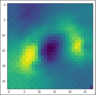
Plot the necessary images to get the training and testing data defined in perfect way using the below code −
pylab.imshow(img, cmap ='gray')
pylab.axis('off')
pylab.show()
The output is displayed as below −
PyTorch - Sequence Processing with Convents
In this chapter, we propose an alternative approach which instead relies on a single 2D convolutional neural network across both sequences. Each layer of our network re-codes source tokens on the basis of the output sequence produced so far. Attention-like properties are therefore pervasive throughout the network.
Here, we will focus on creating the sequential network with specific pooling from the values included in dataset. This process is also best applied in “Image Recognition Module”.
Following steps are used to create a sequence processing model with convents using PyTorch −
Step 1
Import the necessary modules for performance of sequence processing using convents.
import keras
from keras.datasets import mnist
from keras.models import Sequential
from keras.layers import Dense, Dropout, Flatten
from keras.layers import Conv2D, MaxPooling2D
import numpy as np
Step 2
Perform the necessary operations to create a pattern in respective sequence using the below code −
batch_size = 128
num_classes = 10
epochs = 12
# input image dimensions
img_rows, img_cols = 28, 28
# the data, split between train and test sets
(x_train, y_train), (x_test, y_test) = mnist.load_data()
x_train = x_train.reshape(60000,28,28,1)
x_test = x_test.reshape(10000,28,28,1)
print('x_train shape:', x_train.shape)
print(x_train.shape[0], 'train samples')
print(x_test.shape[0], 'test samples')
y_train = keras.utils.to_categorical(y_train, num_classes)
y_test = keras.utils.to_categorical(y_test, num_classes)
Step 3
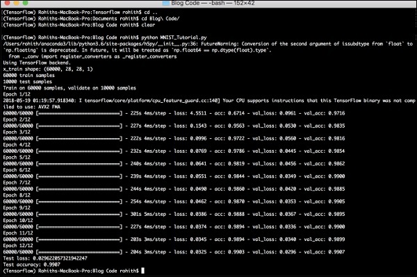
Compile the model and fit the pattern in the mentioned conventional neural network model as shown below −
model.compile(loss =
keras.losses.categorical_crossentropy,
optimizer = keras.optimizers.Adadelta(), metrics =
['accuracy'])
model.fit(x_train, y_train,
batch_size = batch_size, epochs = epochs,
verbose = 1, validation_data = (x_test, y_test))
score = model.evaluate(x_test, y_test, verbose = 0)
print('Test loss:', score[0])
print('Test accuracy:', score[1])
The output generated is as follows −
PyTorch - Word Embedding
In this chapter, we will understand the famous word embedding model − word2vec. Word2vec model is used to produce word embedding with the help of group of related models. Word2vec model is implemented with pure C-code and the gradient are computed manually.
The implementation of word2vec model in PyTorch is explained in the below steps −
Step 1
Implement the libraries in word embedding as mentioned below −
import torch
from torch.autograd import Variable
import torch.nn as nn
import torch.nn.functional as F
Step 2
Implement the Skip Gram Model of word embedding with the class called word2vec. It includes emb_size, emb_dimension, u_embedding, v_embedding type of attributes.
class SkipGramModel(nn.Module):
   def __init__(self, emb_size, emb_dimension):
      super(SkipGramModel, self).__init__()
      self.emb_size = emb_size
      self.emb_dimension = emb_dimension
      self.u_embeddings = nn.Embedding(emb_size, emb_dimension, sparse=True)
      self.v_embeddings = nn.Embedding(emb_size, emb_dimension, sparse = True)
      self.init_emb()
   def init_emb(self):
      initrange = 0.5 / self.emb_dimension
      self.u_embeddings.weight.data.uniform_(-initrange, initrange)
      self.v_embeddings.weight.data.uniform_(-0, 0)
   def forward(self, pos_u, pos_v, neg_v):
      emb_u = self.u_embeddings(pos_u)
      emb_v = self.v_embeddings(pos_v)
      score = torch.mul(emb_u, emb_v).squeeze()
      score = torch.sum(score, dim = 1)
      score = F.logsigmoid(score)
      neg_emb_v = self.v_embeddings(neg_v)
      neg_score = torch.bmm(neg_emb_v, emb_u.unsqueeze(2)).squeeze()
      neg_score = F.logsigmoid(-1 * neg_score)
      return -1 * (torch.sum(score)+torch.sum(neg_score))
   def save_embedding(self, id2word, file_name, use_cuda):
      if use_cuda:
         embedding = self.u_embeddings.weight.cpu().data.numpy()
      else:
         embedding = self.u_embeddings.weight.data.numpy()
      fout = open(file_name, 'w')
      fout.write('%d %d\n' % (len(id2word), self.emb_dimension))
      for wid, w in id2word.items():
         e = embedding[wid]
         e = ' '.join(map(lambda x: str(x), e))
         fout.write('%s %s\n' % (w, e))
def test():
   model = SkipGramModel(100, 100)
   id2word = dict()
   for i in range(100):
      id2word[i] = str(i)
   model.save_embedding(id2word)
Step 3
Implement the main method to get the word embedding model displayed in proper way.
if __name__  ==  '__main__':
   test()
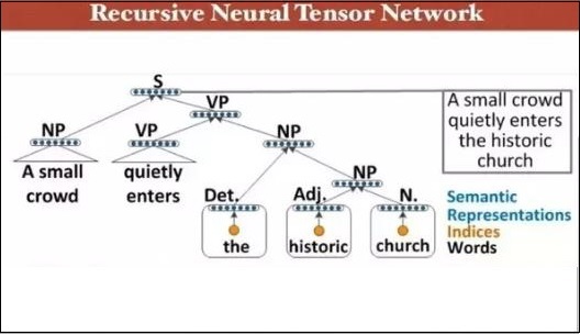
PyTorch - Recursive Neural Networks
Deep neural networks have an exclusive feature for enabling breakthroughs in machine learning understanding the process of natural language. It is observed that most of these models treat language as a flat sequence of words or characters, and use a kind of model which is referred as recurrent neural network or RNN.
Many researchers come to a conclusion that language is best understood with respect to hierarchical tree of phrases. This type is included in recursive neural networks that take a specific structure into account.
PyTorch has a specific feature which helps to make these complex natural language processing models a lot easier. It is a fully-featured framework for all kinds of deep learning with strong support for computer vision.
Features of Recursive Neural Network
A recursive neural network is created in such a way that it includes applying same set of weights with different graph like structures.
The nodes are traversed in topological order.
This type of network is trained by the reverse mode of automatic differentiation.
Natural language processing includes a special case of recursive neural networks.
This recursive neural tensor network includes various composition functional nodes in the tree.
The example of recursive neural network is demonstrated below −