- Python Pandas Tutorial
- Python Pandas - Home
- Python Pandas - Introduction
- Python Pandas - Environment Setup
- Introduction to Data Structures
- Python Pandas - Series
- Python Pandas - DataFrame
- Python Pandas - Panel
- Python Pandas - Basic Functionality
- Descriptive Statistics
- Function Application
- Python Pandas - Reindexing
- Python Pandas - Iteration
- Python Pandas - Sorting
- Working with Text Data
- Options & Customization
- Indexing & Selecting Data
- Statistical Functions
- Python Pandas - Window Functions
- Python Pandas - Aggregations
- Python Pandas - Missing Data
- Python Pandas - GroupBy
- Python Pandas - Merging/Joining
- Python Pandas - Concatenation
- Python Pandas - Date Functionality
- Python Pandas - Timedelta
- Python Pandas - Categorical Data
- Python Pandas - Visualization
- Python Pandas - IO Tools
- Python Pandas - Sparse Data
- Python Pandas - Caveats & Gotchas
- Comparison with SQL
- Python Pandas Useful Resources
- Python Pandas - Quick Guide
- Python Pandas - Useful Resources
- Python Pandas - Discussion
Python Pandas - Quick Guide
Python Pandas - Introduction
Pandas is an open-source Python Library providing high-performance data manipulation and analysis tool using its powerful data structures. The name Pandas is derived from the word Panel Data – an Econometrics from Multidimensional data.
In 2008, developer Wes McKinney started developing pandas when in need of high performance, flexible tool for analysis of data.
Prior to Pandas, Python was majorly used for data munging and preparation. It had very little contribution towards data analysis. Pandas solved this problem. Using Pandas, we can accomplish five typical steps in the processing and analysis of data, regardless of the origin of data — load, prepare, manipulate, model, and analyze.
Python with Pandas is used in a wide range of fields including academic and commercial domains including finance, economics, Statistics, analytics, etc.
Key Features of Pandas
- Fast and efficient DataFrame object with default and customized indexing.
- Tools for loading data into in-memory data objects from different file formats.
- Data alignment and integrated handling of missing data.
- Reshaping and pivoting of date sets.
- Label-based slicing, indexing and subsetting of large data sets.
- Columns from a data structure can be deleted or inserted.
- Group by data for aggregation and transformations.
- High performance merging and joining of data.
- Time Series functionality.
Python Pandas - Environment Setup
Standard Python distribution doesn't come bundled with Pandas module. A lightweight alternative is to install NumPy using popular Python package installer, pip.
pip install pandas
If you install Anaconda Python package, Pandas will be installed by default with the following −
Windows
Anaconda (from https://www.continuum.io) is a free Python distribution for SciPy stack. It is also available for Linux and Mac.
Canopy (https://www.enthought.com/products/canopy/) is available as free as well as commercial distribution with full SciPy stack for Windows, Linux and Mac.
Python (x,y) is a free Python distribution with SciPy stack and Spyder IDE for Windows OS. (Downloadable from http://python-xy.github.io/)
Linux
Package managers of respective Linux distributions are used to install one or more packages in SciPy stack.
For Ubuntu Users
sudo apt-get install python-numpy python-scipy python-matplotlibipythonipythonnotebook
python-pandas python-sympy python-nose
For Fedora Users
sudo yum install numpyscipy python-matplotlibipython python-pandas sympy
python-nose atlas-devel
Introduction to Data Structures
Pandas deals with the following three data structures −
- Series
- DataFrame
- Panel
These data structures are built on top of Numpy array, which means they are fast.
Dimension & Description
The best way to think of these data structures is that the higher dimensional data structure is a container of its lower dimensional data structure. For example, DataFrame is a container of Series, Panel is a container of DataFrame.
| Data Structure | Dimensions | Description |
|---|---|---|
| Series | 1 | 1D labeled homogeneous array, sizeimmutable. |
| Data Frames | 2 | General 2D labeled, size-mutable tabular structure with potentially heterogeneously typed columns. |
| Panel | 3 | General 3D labeled, size-mutable array. |
Building and handling two or more dimensional arrays is a tedious task, burden is placed on the user to consider the orientation of the data set when writing functions. But using Pandas data structures, the mental effort of the user is reduced.
For example, with tabular data (DataFrame) it is more semantically helpful to think of the index (the rows) and the columns rather than axis 0 and axis 1.
Mutability
All Pandas data structures are value mutable (can be changed) and except Series all are size mutable. Series is size immutable.
Note − DataFrame is widely used and one of the most important data structures. Panel is used much less.
Series
Series is a one-dimensional array like structure with homogeneous data. For example, the following series is a collection of integers 10, 23, 56, …
| 10 | 23 | 56 | 17 | 52 | 61 | 73 | 90 | 26 | 72 |
Key Points
- Homogeneous data
- Size Immutable
- Values of Data Mutable
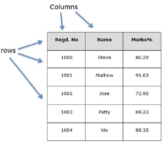
DataFrame
DataFrame is a two-dimensional array with heterogeneous data. For example,
| Name | Age | Gender | Rating |
|---|---|---|---|
| Steve | 32 | Male | 3.45 |
| Lia | 28 | Female | 4.6 |
| Vin | 45 | Male | 3.9 |
| Katie | 38 | Female | 2.78 |
The table represents the data of a sales team of an organization with their overall performance rating. The data is represented in rows and columns. Each column represents an attribute and each row represents a person.
Data Type of Columns
The data types of the four columns are as follows −
| Column | Type |
|---|---|
| Name | String |
| Age | Integer |
| Gender | String |
| Rating | Float |
Key Points
- Heterogeneous data
- Size Mutable
- Data Mutable
Panel
Panel is a three-dimensional data structure with heterogeneous data. It is hard to represent the panel in graphical representation. But a panel can be illustrated as a container of DataFrame.
Key Points
- Heterogeneous data
- Size Mutable
- Data Mutable
Python Pandas - Series
Series is a one-dimensional labeled array capable of holding data of any type (integer, string, float, python objects, etc.). The axis labels are collectively called index.
pandas.Series
A pandas Series can be created using the following constructor −
pandas.Series( data, index, dtype, copy)
The parameters of the constructor are as follows −
| Sr.No | Parameter & Description |
|---|---|
| 1 |
data data takes various forms like ndarray, list, constants |
| 2 |
index Index values must be unique and hashable, same length as data. Default np.arange(n) if no index is passed. |
| 3 |
dtype dtype is for data type. If None, data type will be inferred |
| 4 |
copy Copy data. Default False |
A series can be created using various inputs like −
- Array
- Dict
- Scalar value or constant
Create an Empty Series
A basic series, which can be created is an Empty Series.
Example
#import the pandas library and aliasing as pd
import pandas as pd
s = pd.Series()
print s
Its output is as follows −
Series([], dtype: float64)
Create a Series from ndarray
If data is an ndarray, then index passed must be of the same length. If no index is passed, then by default index will be range(n) where n is array length, i.e., [0,1,2,3…. range(len(array))-1].
Example 1
#import the pandas library and aliasing as pd
import pandas as pd
import numpy as np
data = np.array(['a','b','c','d'])
s = pd.Series(data)
print s
Its output is as follows −
0   a
1   b
2   c
3   d
dtype: object
We did not pass any index, so by default, it assigned the indexes ranging from 0 to len(data)-1, i.e., 0 to 3.
Example 2
#import the pandas library and aliasing as pd
import pandas as pd
import numpy as np
data = np.array(['a','b','c','d'])
s = pd.Series(data,index=[100,101,102,103])
print s
Its output is as follows −
100  a
101  b
102  c
103  d
dtype: object
We passed the index values here. Now we can see the customized indexed values in the output.
Create a Series from dict
A dict can be passed as input and if no index is specified, then the dictionary keys are taken in a sorted order to construct index. If index is passed, the values in data corresponding to the labels in the index will be pulled out.
Example 1
#import the pandas library and aliasing as pd
import pandas as pd
import numpy as np
data = {'a' : 0., 'b' : 1., 'c' : 2.}
s = pd.Series(data)
print s
Its output is as follows −
a 0.0
b 1.0
c 2.0
dtype: float64
Observe − Dictionary keys are used to construct index.
Example 2
#import the pandas library and aliasing as pd
import pandas as pd
import numpy as np
data = {'a' : 0., 'b' : 1., 'c' : 2.}
s = pd.Series(data,index=['b','c','d','a'])
print s
Its output is as follows −
b 1.0
c 2.0
d NaN
a 0.0
dtype: float64
Observe − Index order is persisted and the missing element is filled with NaN (Not a Number).
Create a Series from Scalar
If data is a scalar value, an index must be provided. The value will be repeated to match the length of index
#import the pandas library and aliasing as pd
import pandas as pd
import numpy as np
s = pd.Series(5, index=[0, 1, 2, 3])
print s
Its output is as follows −
0  5
1  5
2  5
3  5
dtype: int64
Accessing Data from Series with Position
Data in the series can be accessed similar to that in an ndarray.
Example 1
Retrieve the first element. As we already know, the counting starts from zero for the array, which means the first element is stored at zeroth position and so on.
import pandas as pd
s = pd.Series([1,2,3,4,5],index = ['a','b','c','d','e'])

#retrieve the first element
print s[0]
Its output is as follows −
1
Example 2
Retrieve the first three elements in the Series. If a : is inserted in front of it, all items from that index onwards will be extracted. If two parameters (with : between them) is used, items between the two indexes (not including the stop index)
import pandas as pd
s = pd.Series([1,2,3,4,5],index = ['a','b','c','d','e'])

#retrieve the first three element
print s[:3]
Its output is as follows −
a  1
b  2
c  3
dtype: int64
Example 3
Retrieve the last three elements.
import pandas as pd
s = pd.Series([1,2,3,4,5],index = ['a','b','c','d','e'])

#retrieve the last three element
print s[-3:]
Its output is as follows −
c  3
d  4
e  5
dtype: int64
Retrieve Data Using Label (Index)
A Series is like a fixed-size dict in that you can get and set values by index label.
Example 1
Retrieve a single element using index label value.
import pandas as pd
s = pd.Series([1,2,3,4,5],index = ['a','b','c','d','e'])

#retrieve a single element
print s['a']
Its output is as follows −
1
Example 2
Retrieve multiple elements using a list of index label values.
import pandas as pd
s = pd.Series([1,2,3,4,5],index = ['a','b','c','d','e'])

#retrieve multiple elements
print s[['a','c','d']]
Its output is as follows −
a  1
c  3
d  4
dtype: int64
Example 3
If a label is not contained, an exception is raised.
import pandas as pd
s = pd.Series([1,2,3,4,5],index = ['a','b','c','d','e'])

#retrieve multiple elements
print s['f']
Its output is as follows −
…
KeyError: 'f'
Python Pandas - DataFrame
A Data frame is a two-dimensional data structure, i.e., data is aligned in a tabular fashion in rows and columns.
Features of DataFrame
- Potentially columns are of different types
- Size – Mutable
- Labeled axes (rows and columns)
- Can Perform Arithmetic operations on rows and columns
Structure
Let us assume that we are creating a data frame with student’s data.
You can think of it as an SQL table or a spreadsheet data representation.
pandas.DataFrame
A pandas DataFrame can be created using the following constructor −
pandas.DataFrame( data, index, columns, dtype, copy)
The parameters of the constructor are as follows −
| Sr.No | Parameter & Description |
|---|---|
| 1 |
data data takes various forms like ndarray, series, map, lists, dict, constants and also another DataFrame. |
| 2 |
index For the row labels, the Index to be used for the resulting frame is Optional Default np.arange(n) if no index is passed. |
| 3 |
columns For column labels, the optional default syntax is - np.arange(n). This is only true if no index is passed. |
| 4 |
dtype Data type of each column. |
| 5 |
copy This command (or whatever it is) is used for copying of data, if the default is False. |
Create DataFrame
A pandas DataFrame can be created using various inputs like −
- Lists
- dict
- Series
- Numpy ndarrays
- Another DataFrame
In the subsequent sections of this chapter, we will see how to create a DataFrame using these inputs.
Create an Empty DataFrame
A basic DataFrame, which can be created is an Empty Dataframe.
Example
#import the pandas library and aliasing as pd
import pandas as pd
df = pd.DataFrame()
print df
Its output is as follows −
Empty DataFrame
Columns: []
Index: []
Create a DataFrame from Lists
The DataFrame can be created using a single list or a list of lists.
Example 1
import pandas as pd
data = [1,2,3,4,5]
df = pd.DataFrame(data)
print df
Its output is as follows −
     0
0    1
1    2
2    3
3    4
4    5
Example 2
import pandas as pd
data = [['Alex',10],['Bob',12],['Clarke',13]]
df = pd.DataFrame(data,columns=['Name','Age'])
print df
Its output is as follows −
      Name      Age
0     Alex      10
1     Bob       12
2     Clarke    13
Example 3
import pandas as pd
data = [['Alex',10],['Bob',12],['Clarke',13]]
df = pd.DataFrame(data,columns=['Name','Age'],dtype=float)
print df
Its output is as follows −
      Name     Age
0     Alex     10.0
1     Bob      12.0
2     Clarke   13.0
Note − Observe, the dtype parameter changes the type of Age column to floating point.
Create a DataFrame from Dict of ndarrays / Lists
All the ndarrays must be of same length. If index is passed, then the length of the index should equal to the length of the arrays.
If no index is passed, then by default, index will be range(n), where n is the array length.
Example 1
import pandas as pd
data = {'Name':['Tom', 'Jack', 'Steve', 'Ricky'],'Age':[28,34,29,42]}
df = pd.DataFrame(data)
print df
Its output is as follows −
      Age      Name
0     28        Tom
1     34       Jack
2     29      Steve
3     42      Ricky
Note − Observe the values 0,1,2,3. They are the default index assigned to each using the function range(n).
Example 2
Let us now create an indexed DataFrame using arrays.
import pandas as pd
data = {'Name':['Tom', 'Jack', 'Steve', 'Ricky'],'Age':[28,34,29,42]}
df = pd.DataFrame(data, index=['rank1','rank2','rank3','rank4'])
print df
Its output is as follows −
         Age    Name
rank1    28      Tom
rank2    34     Jack
rank3    29    Steve
rank4    42    Ricky
Note − Observe, the index parameter assigns an index to each row.
Create a DataFrame from List of Dicts
List of Dictionaries can be passed as input data to create a DataFrame. The dictionary keys are by default taken as column names.
Example 1
The following example shows how to create a DataFrame by passing a list of dictionaries.
import pandas as pd
data = [{'a': 1, 'b': 2},{'a': 5, 'b': 10, 'c': 20}]
df = pd.DataFrame(data)
print df
Its output is as follows −
    a    b      c
0   1   2     NaN
1   5   10   20.0
Note − Observe, NaN (Not a Number) is appended in missing areas.
Example 2
The following example shows how to create a DataFrame by passing a list of dictionaries and the row indices.
import pandas as pd
data = [{'a': 1, 'b': 2},{'a': 5, 'b': 10, 'c': 20}]
df = pd.DataFrame(data, index=['first', 'second'])
print df
Its output is as follows −
        a   b       c
first   1   2     NaN
second  5   10   20.0
Example 3
The following example shows how to create a DataFrame with a list of dictionaries, row indices, and column indices.
import pandas as pd
data = [{'a': 1, 'b': 2},{'a': 5, 'b': 10, 'c': 20}]

#With two column indices, values same as dictionary keys
df1 = pd.DataFrame(data, index=['first', 'second'], columns=['a', 'b'])

#With two column indices with one index with other name
df2 = pd.DataFrame(data, index=['first', 'second'], columns=['a', 'b1'])
print df1
print df2
Its output is as follows −
#df1 output
         a  b
first    1  2
second   5  10

#df2 output
         a  b1
first    1  NaN
second   5  NaN
Note − Observe, df2 DataFrame is created with a column index other than the dictionary key; thus, appended the NaN’s in place. Whereas, df1 is created with column indices same as dictionary keys, so NaN’s appended.
Create a DataFrame from Dict of Series
Dictionary of Series can be passed to form a DataFrame. The resultant index is the union of all the series indexes passed.
Example
import pandas as pd

d = {'one' : pd.Series([1, 2, 3], index=['a', 'b', 'c']),
   'two' : pd.Series([1, 2, 3, 4], index=['a', 'b', 'c', 'd'])}

df = pd.DataFrame(d)
print df
Its output is as follows −
      one    two
a     1.0    1
b     2.0    2
c     3.0    3
d     NaN    4
Note − Observe, for the series one, there is no label ‘d’ passed, but in the result, for the d label, NaN is appended with NaN.
Let us now understand column selection, addition, and deletion through examples.
Column Selection
We will understand this by selecting a column from the DataFrame.
Example
import pandas as pd

d = {'one' : pd.Series([1, 2, 3], index=['a', 'b', 'c']),
   'two' : pd.Series([1, 2, 3, 4], index=['a', 'b', 'c', 'd'])}

df = pd.DataFrame(d)
print df ['one']
Its output is as follows −
a     1.0
b     2.0
c     3.0
d     NaN
Name: one, dtype: float64
Column Addition
We will understand this by adding a new column to an existing data frame.
Example
import pandas as pd

d = {'one' : pd.Series([1, 2, 3], index=['a', 'b', 'c']),
   'two' : pd.Series([1, 2, 3, 4], index=['a', 'b', 'c', 'd'])}

df = pd.DataFrame(d)

# Adding a new column to an existing DataFrame object with column label by passing new series

print ("Adding a new column by passing as Series:")
df['three']=pd.Series([10,20,30],index=['a','b','c'])
print df

print ("Adding a new column using the existing columns in DataFrame:")
df['four']=df['one']+df['three']

print df
Its output is as follows −
Adding a new column by passing as Series:
     one   two   three
a    1.0    1    10.0
b    2.0    2    20.0
c    3.0    3    30.0
d    NaN    4    NaN

Adding a new column using the existing columns in DataFrame:
      one   two   three    four
a     1.0    1    10.0     11.0
b     2.0    2    20.0     22.0
c     3.0    3    30.0     33.0
d     NaN    4     NaN     NaN
Column Deletion
Columns can be deleted or popped; let us take an example to understand how.
Example
# Using the previous DataFrame, we will delete a column
# using del function
import pandas as pd

d = {'one' : pd.Series([1, 2, 3], index=['a', 'b', 'c']),
   'two' : pd.Series([1, 2, 3, 4], index=['a', 'b', 'c', 'd']),
   'three' : pd.Series([10,20,30], index=['a','b','c'])}

df = pd.DataFrame(d)
print ("Our dataframe is:")
print df

# using del function
print ("Deleting the first column using DEL function:")
del df['one']
print df

# using pop function
print ("Deleting another column using POP function:")
df.pop('two')
print df
Its output is as follows −
Our dataframe is:
      one   three  two
a     1.0    10.0   1
b     2.0    20.0   2
c     3.0    30.0   3
d     NaN     NaN   4

Deleting the first column using DEL function:
      three    two
a     10.0     1
b     20.0     2
c     30.0     3
d     NaN      4

Deleting another column using POP function:
   three
a  10.0
b  20.0
c  30.0
d  NaN
Row Selection, Addition, and Deletion
We will now understand row selection, addition and deletion through examples. Let us begin with the concept of selection.
Selection by Label
Rows can be selected by passing row label to a loc function.
import pandas as pd

d = {'one' : pd.Series([1, 2, 3], index=['a', 'b', 'c']),
   'two' : pd.Series([1, 2, 3, 4], index=['a', 'b', 'c', 'd'])}

df = pd.DataFrame(d)
print df.loc['b']
Its output is as follows −
one 2.0
two 2.0
Name: b, dtype: float64
The result is a series with labels as column names of the DataFrame. And, the Name of the series is the label with which it is retrieved.
Selection by integer location
Rows can be selected by passing integer location to an iloc function.
import pandas as pd

d = {'one' : pd.Series([1, 2, 3], index=['a', 'b', 'c']),
   'two' : pd.Series([1, 2, 3, 4], index=['a', 'b', 'c', 'd'])}

df = pd.DataFrame(d)
print df.iloc[2]
Its output is as follows −
one   3.0
two   3.0
Name: c, dtype: float64
Slice Rows
Multiple rows can be selected using ‘ : ’ operator.
import pandas as pd

d = {'one' : pd.Series([1, 2, 3], index=['a', 'b', 'c']),
   'two' : pd.Series([1, 2, 3, 4], index=['a', 'b', 'c', 'd'])}

df = pd.DataFrame(d)
print df[2:4]
Its output is as follows −
   one  two
c  3.0    3
d  NaN    4
Addition of Rows
Add new rows to a DataFrame using the append function. This function will append the rows at the end.
import pandas as pd

df = pd.DataFrame([[1, 2], [3, 4]], columns = ['a','b'])
df2 = pd.DataFrame([[5, 6], [7, 8]], columns = ['a','b'])

df = df.append(df2)
print df
Its output is as follows −
   a  b
0  1  2
1  3  4
0  5  6
1  7  8
Deletion of Rows
Use index label to delete or drop rows from a DataFrame. If label is duplicated, then multiple rows will be dropped.
If you observe, in the above example, the labels are duplicate. Let us drop a label and will see how many rows will get dropped.
import pandas as pd

df = pd.DataFrame([[1, 2], [3, 4]], columns = ['a','b'])
df2 = pd.DataFrame([[5, 6], [7, 8]], columns = ['a','b'])

df = df.append(df2)

# Drop rows with label 0
df = df.drop(0)

print df
Its output is as follows −
  a b
1 3 4
1 7 8
In the above example, two rows were dropped because those two contain the same label 0.
Python Pandas - Panel
A panel is a 3D container of data. The term Panel data is derived from econometrics and is partially responsible for the name pandas − pan(el)-da(ta)-s.
The names for the 3 axes are intended to give some semantic meaning to describing operations involving panel data. They are −
items − axis 0, each item corresponds to a DataFrame contained inside.
major_axis − axis 1, it is the index (rows) of each of the DataFrames.
minor_axis − axis 2, it is the columns of each of the DataFrames.
pandas.Panel()
A Panel can be created using the following constructor −
pandas.Panel(data, items, major_axis, minor_axis, dtype, copy)
The parameters of the constructor are as follows −
| Parameter | Description |
|---|---|
| data | Data takes various forms like ndarray, series, map, lists, dict, constants and also another DataFrame |
| items | axis=0 |
| major_axis | axis=1 |
| minor_axis | axis=2 |
| dtype | Data type of each column |
| copy | Copy data. Default, false |
Create Panel
A Panel can be created using multiple ways like −
- From ndarrays
- From dict of DataFrames
From 3D ndarray
# creating an empty panel
import pandas as pd
import numpy as np

data = np.random.rand(2,4,5)
p = pd.Panel(data)
print p
Its output is as follows −
<class 'pandas.core.panel.Panel'>
Dimensions: 2 (items) x 4 (major_axis) x 5 (minor_axis)
Items axis: 0 to 1
Major_axis axis: 0 to 3
Minor_axis axis: 0 to 4
Note − Observe the dimensions of the empty panel and the above panel, all the objects are different.
From dict of DataFrame Objects
#creating an empty panel
import pandas as pd
import numpy as np

data = {'Item1' : pd.DataFrame(np.random.randn(4, 3)),
   'Item2' : pd.DataFrame(np.random.randn(4, 2))}
p = pd.Panel(data)
print p
Its output is as follows −
Dimensions: 2 (items) x 4 (major_axis) x 3 (minor_axis)
Items axis: Item1 to Item2
Major_axis axis: 0 to 3
Minor_axis axis: 0 to 2
Create an Empty Panel
An empty panel can be created using the Panel constructor as follows −
#creating an empty panel
import pandas as pd
p = pd.Panel()
print p
Its output is as follows −
<class 'pandas.core.panel.Panel'>
Dimensions: 0 (items) x 0 (major_axis) x 0 (minor_axis)
Items axis: None
Major_axis axis: None
Minor_axis axis: None
Selecting the Data from Panel
Select the data from the panel using −
- Items
- Major_axis
- Minor_axis
Using Items
# creating an empty panel
import pandas as pd
import numpy as np
data = {'Item1' : pd.DataFrame(np.random.randn(4, 3)),
   'Item2' : pd.DataFrame(np.random.randn(4, 2))}
p = pd.Panel(data)
print p['Item1']
Its output is as follows −
            0          1          2
0    0.488224  -0.128637   0.930817
1    0.417497   0.896681   0.576657
2   -2.775266   0.571668   0.290082
3   -0.400538  -0.144234   1.110535
We have two items, and we retrieved item1. The result is a DataFrame with 4 rows and 3 columns, which are the Major_axis and Minor_axis dimensions.
Using major_axis
Data can be accessed using the method panel.major_axis(index).
# creating an empty panel
import pandas as pd
import numpy as np
data = {'Item1' : pd.DataFrame(np.random.randn(4, 3)),
   'Item2' : pd.DataFrame(np.random.randn(4, 2))}
p = pd.Panel(data)
print p.major_xs(1)
Its output is as follows −
      Item1       Item2
0   0.417497    0.748412
1   0.896681   -0.557322
2   0.576657       NaN
Using minor_axis
Data can be accessed using the method panel.minor_axis(index).
# creating an empty panel
import pandas as pd
import numpy as np
data = {'Item1' : pd.DataFrame(np.random.randn(4, 3)),
   'Item2' : pd.DataFrame(np.random.randn(4, 2))}
p = pd.Panel(data)
print p.minor_xs(1)
Its output is as follows −
       Item1       Item2
0   -0.128637   -1.047032
1    0.896681   -0.557322
2    0.571668    0.431953
3   -0.144234    1.302466
Note − Observe the changes in the dimensions.
Python Pandas - Basic Functionality
By now, we learnt about the three Pandas DataStructures and how to create them. We will majorly focus on the DataFrame objects because of its importance in the real time data processing and also discuss a few other DataStructures.
Series Basic Functionality
| Sr.No. | Attribute or Method & Description |
|---|---|
| 1 |
axes Returns a list of the row axis labels |
| 2 |
dtype Returns the dtype of the object. |
| 3 |
empty Returns True if series is empty. |
| 4 |
ndim Returns the number of dimensions of the underlying data, by definition 1. |
| 5 |
size Returns the number of elements in the underlying data. |
| 6 |
values Returns the Series as ndarray. |
| 7 |
head() Returns the first n rows. |
| 8 |
tail() Returns the last n rows. |
Let us now create a Series and see all the above tabulated attributes operation.
Example
import pandas as pd
import numpy as np

#Create a series with 100 random numbers
s = pd.Series(np.random.randn(4))
print s
Its output is as follows −
0   0.967853
1  -0.148368
2  -1.395906
3  -1.758394
dtype: float64
axes
Returns the list of the labels of the series.
import pandas as pd
import numpy as np

#Create a series with 100 random numbers
s = pd.Series(np.random.randn(4))
print ("The axes are:")
print s.axes
Its output is as follows −
The axes are:
[RangeIndex(start=0, stop=4, step=1)]
The above result is a compact format of a list of values from 0 to 5, i.e., [0,1,2,3,4].
empty
Returns the Boolean value saying whether the Object is empty or not. True indicates that the object is empty.
import pandas as pd
import numpy as np

#Create a series with 100 random numbers
s = pd.Series(np.random.randn(4))
print ("Is the Object empty?")
print s.empty
Its output is as follows −
Is the Object empty?
False
ndim
Returns the number of dimensions of the object. By definition, a Series is a 1D data structure, so it returns
import pandas as pd
import numpy as np

#Create a series with 4 random numbers
s = pd.Series(np.random.randn(4))
print s

print ("The dimensions of the object:")
print s.ndim
Its output is as follows −
0   0.175898
1   0.166197
2  -0.609712
3  -1.377000
dtype: float64

The dimensions of the object:
1
size
Returns the size(length) of the series.
import pandas as pd
import numpy as np

#Create a series with 4 random numbers
s = pd.Series(np.random.randn(2))
print s
print ("The size of the object:")
print s.size
Its output is as follows −
0   3.078058
1  -1.207803
dtype: float64

The size of the object:
2
values
Returns the actual data in the series as an array.
import pandas as pd
import numpy as np

#Create a series with 4 random numbers
s = pd.Series(np.random.randn(4))
print s

print ("The actual data series is:")
print s.values
Its output is as follows −
0   1.787373
1  -0.605159
2   0.180477
3  -0.140922
dtype: float64

The actual data series is:
[ 1.78737302 -0.60515881 0.18047664 -0.1409218 ]
Head & Tail
To view a small sample of a Series or the DataFrame object, use the head() and the tail() methods.
head() returns the first n rows(observe the index values). The default number of elements to display is five, but you may pass a custom number.
import pandas as pd
import numpy as np

#Create a series with 4 random numbers
s = pd.Series(np.random.randn(4))
print ("The original series is:")
print s

print ("The first two rows of the data series:")
print s.head(2)
Its output is as follows −
The original series is:
0   0.720876
1  -0.765898
2   0.479221
3  -0.139547
dtype: float64

The first two rows of the data series:
0   0.720876
1  -0.765898
dtype: float64
tail() returns the last n rows(observe the index values). The default number of elements to display is five, but you may pass a custom number.
import pandas as pd
import numpy as np

#Create a series with 4 random numbers
s = pd.Series(np.random.randn(4))
print ("The original series is:")
print s

print ("The last two rows of the data series:")
print s.tail(2)
Its output is as follows −
The original series is:
0 -0.655091
1 -0.881407
2 -0.608592
3 -2.341413
dtype: float64

The last two rows of the data series:
2 -0.608592
3 -2.341413
dtype: float64
DataFrame Basic Functionality
Let us now understand what DataFrame Basic Functionality is. The following tables lists down the important attributes or methods that help in DataFrame Basic Functionality.
| Sr.No. | Attribute or Method & Description |
|---|---|
| 1 |
T Transposes rows and columns. |
| 2 |
axes Returns a list with the row axis labels and column axis labels as the only members. |
| 3 |
dtypes Returns the dtypes in this object. |
| 4 |
empty True if NDFrame is entirely empty [no items]; if any of the axes are of length 0. |
| 5 |
ndim Number of axes / array dimensions. |
| 6 |
shape Returns a tuple representing the dimensionality of the DataFrame. |
| 7 |
size Number of elements in the NDFrame. |
| 8 |
values Numpy representation of NDFrame. |
| 9 |
head() Returns the first n rows. |
| 10 |
tail() Returns last n rows. |
Let us now create a DataFrame and see all how the above mentioned attributes operate.
Example
import pandas as pd
import numpy as np

#Create a Dictionary of series
d = {'Name':pd.Series(['Tom','James','Ricky','Vin','Steve','Smith','Jack']),
   'Age':pd.Series([25,26,25,23,30,29,23]),
   'Rating':pd.Series([4.23,3.24,3.98,2.56,3.20,4.6,3.8])}

#Create a DataFrame
df = pd.DataFrame(d)
print ("Our data series is:")
print df
Its output is as follows −
Our data series is:
    Age   Name    Rating
0   25    Tom     4.23
1   26    James   3.24
2   25    Ricky   3.98
3   23    Vin     2.56
4   30    Steve   3.20
5   29    Smith   4.60
6   23    Jack    3.80
T (Transpose)
Returns the transpose of the DataFrame. The rows and columns will interchange.
import pandas as pd
import numpy as np

# Create a Dictionary of series
d = {'Name':pd.Series(['Tom','James','Ricky','Vin','Steve','Smith','Jack']),
   'Age':pd.Series([25,26,25,23,30,29,23]),
   'Rating':pd.Series([4.23,3.24,3.98,2.56,3.20,4.6,3.8])}

# Create a DataFrame
df = pd.DataFrame(d)
print ("The transpose of the data series is:")
print df.T
Its output is as follows −
The transpose of the data series is:
         0     1       2      3      4      5       6
Age      25    26      25     23     30     29      23
Name     Tom   James   Ricky  Vin    Steve  Smith   Jack
Rating   4.23  3.24    3.98   2.56   3.2    4.6     3.8
axes
Returns the list of row axis labels and column axis labels.
import pandas as pd
import numpy as np

#Create a Dictionary of series
d = {'Name':pd.Series(['Tom','James','Ricky','Vin','Steve','Smith','Jack']),
   'Age':pd.Series([25,26,25,23,30,29,23]),
   'Rating':pd.Series([4.23,3.24,3.98,2.56,3.20,4.6,3.8])}

#Create a DataFrame
df = pd.DataFrame(d)
print ("Row axis labels and column axis labels are:")
print df.axes
Its output is as follows −
Row axis labels and column axis labels are:

[RangeIndex(start=0, stop=7, step=1), Index([u'Age', u'Name', u'Rating'],
dtype='object')]
dtypes
Returns the data type of each column.
import pandas as pd
import numpy as np

#Create a Dictionary of series
d = {'Name':pd.Series(['Tom','James','Ricky','Vin','Steve','Smith','Jack']),
   'Age':pd.Series([25,26,25,23,30,29,23]),
   'Rating':pd.Series([4.23,3.24,3.98,2.56,3.20,4.6,3.8])}

#Create a DataFrame
df = pd.DataFrame(d)
print ("The data types of each column are:")
print df.dtypes
Its output is as follows −
The data types of each column are:
Age     int64
Name    object
Rating  float64
dtype: object
empty
Returns the Boolean value saying whether the Object is empty or not; True indicates that the object is empty.
import pandas as pd
import numpy as np

#Create a Dictionary of series
d = {'Name':pd.Series(['Tom','James','Ricky','Vin','Steve','Smith','Jack']),
   'Age':pd.Series([25,26,25,23,30,29,23]),
   'Rating':pd.Series([4.23,3.24,3.98,2.56,3.20,4.6,3.8])}

#Create a DataFrame
df = pd.DataFrame(d)
print ("Is the object empty?")
print df.empty
Its output is as follows −
Is the object empty?
False
ndim
Returns the number of dimensions of the object. By definition, DataFrame is a 2D object.
import pandas as pd
import numpy as np

#Create a Dictionary of series
d = {'Name':pd.Series(['Tom','James','Ricky','Vin','Steve','Smith','Jack']),
   'Age':pd.Series([25,26,25,23,30,29,23]),
   'Rating':pd.Series([4.23,3.24,3.98,2.56,3.20,4.6,3.8])}

#Create a DataFrame
df = pd.DataFrame(d)
print ("Our object is:")
print df
print ("The dimension of the object is:")
print df.ndim
Its output is as follows −
Our object is:
      Age    Name     Rating
0     25     Tom      4.23
1     26     James    3.24
2     25     Ricky    3.98
3     23     Vin      2.56
4     30     Steve    3.20
5     29     Smith    4.60
6     23     Jack     3.80

The dimension of the object is:
2
shape
Returns a tuple representing the dimensionality of the DataFrame. Tuple (a,b), where a represents the number of rows and b represents the number of columns.
import pandas as pd
import numpy as np

#Create a Dictionary of series
d = {'Name':pd.Series(['Tom','James','Ricky','Vin','Steve','Smith','Jack']),
   'Age':pd.Series([25,26,25,23,30,29,23]),
   'Rating':pd.Series([4.23,3.24,3.98,2.56,3.20,4.6,3.8])}

#Create a DataFrame
df = pd.DataFrame(d)
print ("Our object is:")
print df
print ("The shape of the object is:")
print df.shape
Its output is as follows −
Our object is:
   Age   Name    Rating
0  25    Tom     4.23
1  26    James   3.24
2  25    Ricky   3.98
3  23    Vin     2.56
4  30    Steve   3.20
5  29    Smith   4.60
6  23    Jack    3.80

The shape of the object is:
(7, 3)
size
Returns the number of elements in the DataFrame.
import pandas as pd
import numpy as np

#Create a Dictionary of series
d = {'Name':pd.Series(['Tom','James','Ricky','Vin','Steve','Smith','Jack']),
   'Age':pd.Series([25,26,25,23,30,29,23]),
   'Rating':pd.Series([4.23,3.24,3.98,2.56,3.20,4.6,3.8])}

#Create a DataFrame
df = pd.DataFrame(d)
print ("Our object is:")
print df
print ("The total number of elements in our object is:")
print df.size
Its output is as follows −
Our object is:
    Age   Name    Rating
0   25    Tom     4.23
1   26    James   3.24
2   25    Ricky   3.98
3   23    Vin     2.56
4   30    Steve   3.20
5   29    Smith   4.60
6   23    Jack    3.80

The total number of elements in our object is:
21
values
Returns the actual data in the DataFrame as an NDarray.
import pandas as pd
import numpy as np

#Create a Dictionary of series
d = {'Name':pd.Series(['Tom','James','Ricky','Vin','Steve','Smith','Jack']),
   'Age':pd.Series([25,26,25,23,30,29,23]),
   'Rating':pd.Series([4.23,3.24,3.98,2.56,3.20,4.6,3.8])}

#Create a DataFrame
df = pd.DataFrame(d)
print ("Our object is:")
print df
print ("The actual data in our data frame is:")
print df.values
Its output is as follows −
Our object is:
    Age   Name    Rating
0   25    Tom     4.23
1   26    James   3.24
2   25    Ricky   3.98
3   23    Vin     2.56
4   30    Steve   3.20
5   29    Smith   4.60
6   23    Jack    3.80
The actual data in our data frame is:
[[25 'Tom' 4.23]
[26 'James' 3.24]
[25 'Ricky' 3.98]
[23 'Vin' 2.56]
[30 'Steve' 3.2]
[29 'Smith' 4.6]
[23 'Jack' 3.8]]
Head & Tail
To view a small sample of a DataFrame object, use the head() and tail() methods. head() returns the first n rows (observe the index values). The default number of elements to display is five, but you may pass a custom number.
import pandas as pd
import numpy as np

#Create a Dictionary of series
d = {'Name':pd.Series(['Tom','James','Ricky','Vin','Steve','Smith','Jack']),
   'Age':pd.Series([25,26,25,23,30,29,23]),
   'Rating':pd.Series([4.23,3.24,3.98,2.56,3.20,4.6,3.8])}

#Create a DataFrame
df = pd.DataFrame(d)
print ("Our data frame is:")
print df
print ("The first two rows of the data frame is:")
print df.head(2)
Its output is as follows −
Our data frame is:
    Age   Name    Rating
0   25    Tom     4.23
1   26    James   3.24
2   25    Ricky   3.98
3   23    Vin     2.56
4   30    Steve   3.20
5   29    Smith   4.60
6   23    Jack    3.80

The first two rows of the data frame is:
   Age   Name   Rating
0  25    Tom    4.23
1  26    James  3.24
tail() returns the last n rows (observe the index values). The default number of elements to display is five, but you may pass a custom number.
import pandas as pd
import numpy as np

#Create a Dictionary of series
d = {'Name':pd.Series(['Tom','James','Ricky','Vin','Steve','Smith','Jack']),
   'Age':pd.Series([25,26,25,23,30,29,23]),
   'Rating':pd.Series([4.23,3.24,3.98,2.56,3.20,4.6,3.8])}

#Create a DataFrame
df = pd.DataFrame(d)
print ("Our data frame is:")
print df
print ("The last two rows of the data frame is:")
print df.tail(2)
Its output is as follows −
Our data frame is:
    Age   Name    Rating
0   25    Tom     4.23
1   26    James   3.24
2   25    Ricky   3.98
3   23    Vin     2.56
4   30    Steve   3.20
5   29    Smith   4.60
6   23    Jack    3.80

The last two rows of the data frame is:
    Age   Name    Rating
5   29    Smith    4.6
6   23    Jack     3.8
Python Pandas - Descriptive Statistics
A large number of methods collectively compute descriptive statistics and other related operations on DataFrame. Most of these are aggregations like sum(), mean(), but some of them, like sumsum(), produce an object of the same size. Generally speaking, these methods take an axis argument, just like ndarray.{sum, std, ...}, but the axis can be specified by name or integer
DataFrame − “index” (axis=0, default), “columns” (axis=1)
Let us create a DataFrame and use this object throughout this chapter for all the operations.
Example
import pandas as pd
import numpy as np

#Create a Dictionary of series
d = {'Name':pd.Series(['Tom','James','Ricky','Vin','Steve','Smith','Jack',
   'Lee','David','Gasper','Betina','Andres']),
   'Age':pd.Series([25,26,25,23,30,29,23,34,40,30,51,46]),
   'Rating':pd.Series([4.23,3.24,3.98,2.56,3.20,4.6,3.8,3.78,2.98,4.80,4.10,3.65])
}

#Create a DataFrame
df = pd.DataFrame(d)
print df
Its output is as follows −
    Age  Name   Rating
0   25   Tom     4.23
1   26   James   3.24
2   25   Ricky   3.98
3   23   Vin     2.56
4   30   Steve   3.20
5   29   Smith   4.60
6   23   Jack    3.80
7   34   Lee     3.78
8   40   David   2.98
9   30   Gasper  4.80
10  51   Betina  4.10
11  46   Andres  3.65
sum()
Returns the sum of the values for the requested axis. By default, axis is index (axis=0).
import pandas as pd
import numpy as np

#Create a Dictionary of series
d = {'Name':pd.Series(['Tom','James','Ricky','Vin','Steve','Smith','Jack',
   'Lee','David','Gasper','Betina','Andres']),
   'Age':pd.Series([25,26,25,23,30,29,23,34,40,30,51,46]),
   'Rating':pd.Series([4.23,3.24,3.98,2.56,3.20,4.6,3.8,3.78,2.98,4.80,4.10,3.65])
}

#Create a DataFrame
df = pd.DataFrame(d)
print df.sum()
Its output is as follows −
Age                                                    382
Name     TomJamesRickyVinSteveSmithJackLeeDavidGasperBe...
Rating                                               44.92
dtype: object
Each individual column is added individually (Strings are appended).
axis=1
This syntax will give the output as shown below.
import pandas as pd
import numpy as np

#Create a Dictionary of series
d = {'Name':pd.Series(['Tom','James','Ricky','Vin','Steve','Smith','Jack',
   'Lee','David','Gasper','Betina','Andres']),
   'Age':pd.Series([25,26,25,23,30,29,23,34,40,30,51,46]),
   'Rating':pd.Series([4.23,3.24,3.98,2.56,3.20,4.6,3.8,3.78,2.98,4.80,4.10,3.65])
}

#Create a DataFrame
df = pd.DataFrame(d)
print df.sum(1)
Its output is as follows −
0    29.23
1    29.24
2    28.98
3    25.56
4    33.20
5    33.60
6    26.80
7    37.78
8    42.98
9    34.80
10   55.10
11   49.65
dtype: float64
mean()
Returns the average value
import pandas as pd
import numpy as np

#Create a Dictionary of series
d = {'Name':pd.Series(['Tom','James','Ricky','Vin','Steve','Smith','Jack',
   'Lee','David','Gasper','Betina','Andres']),
   'Age':pd.Series([25,26,25,23,30,29,23,34,40,30,51,46]),
   'Rating':pd.Series([4.23,3.24,3.98,2.56,3.20,4.6,3.8,3.78,2.98,4.80,4.10,3.65])
}

#Create a DataFrame
df = pd.DataFrame(d)
print df.mean()
Its output is as follows −
Age       31.833333
Rating     3.743333
dtype: float64
std()
Returns the Bressel standard deviation of the numerical columns.
import pandas as pd
import numpy as np

#Create a Dictionary of series
d = {'Name':pd.Series(['Tom','James','Ricky','Vin','Steve','Smith','Jack',
   'Lee','David','Gasper','Betina','Andres']),
   'Age':pd.Series([25,26,25,23,30,29,23,34,40,30,51,46]),
   'Rating':pd.Series([4.23,3.24,3.98,2.56,3.20,4.6,3.8,3.78,2.98,4.80,4.10,3.65])
}

#Create a DataFrame
df = pd.DataFrame(d)
print df.std()
Its output is as follows −
Age       9.232682
Rating    0.661628
dtype: float64
Functions & Description
Let us now understand the functions under Descriptive Statistics in Python Pandas. The following table list down the important functions −
| Sr.No. | Function | Description |
|---|---|---|
| 1 | count() | Number of non-null observations |
| 2 | sum() | Sum of values |
| 3 | mean() | Mean of Values |
| 4 | median() | Median of Values |
| 5 | mode() | Mode of values |
| 6 | std() | Standard Deviation of the Values |
| 7 | min() | Minimum Value |
| 8 | max() | Maximum Value |
| 9 | abs() | Absolute Value |
| 10 | prod() | Product of Values |
| 11 | cumsum() | Cumulative Sum |
| 12 | cumprod() | Cumulative Product |
Note − Since DataFrame is a Heterogeneous data structure. Generic operations don’t work with all functions.
Functions like sum(), cumsum() work with both numeric and character (or) string data elements without any error. Though n practice, character aggregations are never used generally, these functions do not throw any exception.
Functions like abs(), cumprod() throw exception when the DataFrame contains character or string data because such operations cannot be performed.
Summarizing Data
The describe() function computes a summary of statistics pertaining to the DataFrame columns.
import pandas as pd
import numpy as np

#Create a Dictionary of series
d = {'Name':pd.Series(['Tom','James','Ricky','Vin','Steve','Smith','Jack',
   'Lee','David','Gasper','Betina','Andres']),
   'Age':pd.Series([25,26,25,23,30,29,23,34,40,30,51,46]),
   'Rating':pd.Series([4.23,3.24,3.98,2.56,3.20,4.6,3.8,3.78,2.98,4.80,4.10,3.65])
}

#Create a DataFrame
df = pd.DataFrame(d)
print df.describe()
Its output is as follows −
               Age         Rating
count    12.000000      12.000000
mean     31.833333       3.743333
std       9.232682       0.661628
min      23.000000       2.560000
25%      25.000000       3.230000
50%      29.500000       3.790000
75%      35.500000       4.132500
max      51.000000       4.800000
This function gives the mean, std and IQR values. And, function excludes the character columns and given summary about numeric columns. 'include' is the argument which is used to pass necessary information regarding what columns need to be considered for summarizing. Takes the list of values; by default, 'number'.
- object − Summarizes String columns
- number − Summarizes Numeric columns
- all − Summarizes all columns together (Should not pass it as a list value)
Now, use the following statement in the program and check the output −
import pandas as pd
import numpy as np

#Create a Dictionary of series
d = {'Name':pd.Series(['Tom','James','Ricky','Vin','Steve','Smith','Jack',
   'Lee','David','Gasper','Betina','Andres']),
   'Age':pd.Series([25,26,25,23,30,29,23,34,40,30,51,46]),
   'Rating':pd.Series([4.23,3.24,3.98,2.56,3.20,4.6,3.8,3.78,2.98,4.80,4.10,3.65])
}

#Create a DataFrame
df = pd.DataFrame(d)
print df.describe(include=['object'])
Its output is as follows −
          Name
count       12
unique      12
top      Ricky
freq         1
Now, use the following statement and check the output −
import pandas as pd
import numpy as np

#Create a Dictionary of series
d = {'Name':pd.Series(['Tom','James','Ricky','Vin','Steve','Smith','Jack',
   'Lee','David','Gasper','Betina','Andres']),
   'Age':pd.Series([25,26,25,23,30,29,23,34,40,30,51,46]),
   'Rating':pd.Series([4.23,3.24,3.98,2.56,3.20,4.6,3.8,3.78,2.98,4.80,4.10,3.65])
}

#Create a DataFrame
df = pd.DataFrame(d)
print df. describe(include='all')
Its output is as follows −
          Age          Name       Rating
count   12.000000        12    12.000000
unique        NaN        12          NaN
top           NaN     Ricky          NaN
freq          NaN         1          NaN
mean    31.833333       NaN     3.743333
std      9.232682       NaN     0.661628
min     23.000000       NaN     2.560000
25%     25.000000       NaN     3.230000
50%     29.500000       NaN     3.790000
75%     35.500000       NaN     4.132500
max     51.000000       NaN     4.800000
Python Pandas - Function Application
To apply your own or another library’s functions to Pandas objects, you should be aware of the three important methods. The methods have been discussed below. The appropriate method to use depends on whether your function expects to operate on an entire DataFrame, row- or column-wise, or element wise.
- Table wise Function Application: pipe()
- Row or Column Wise Function Application: apply()
- Element wise Function Application: applymap()
Table-wise Function Application
Custom operations can be performed by passing the function and the appropriate number of parameters as pipe arguments. Thus, operation is performed on the whole DataFrame.
For example, add a value 2 to all the elements in the DataFrame. Then,
adder function
The adder function adds two numeric values as parameters and returns the sum.
def adder(ele1,ele2):
   return ele1+ele2
We will now use the custom function to conduct operation on the DataFrame.
df = pd.DataFrame(np.random.randn(5,3),columns=['col1','col2','col3'])
df.pipe(adder,2)
Let’s see the full program −
import pandas as pd
import numpy as np

def adder(ele1,ele2):
   return ele1+ele2

df = pd.DataFrame(np.random.randn(5,3),columns=['col1','col2','col3'])
df.pipe(adder,2)
print df.apply(np.mean)
Its output is as follows −
        col1       col2       col3
0   2.176704   2.219691   1.509360
1   2.222378   2.422167   3.953921
2   2.241096   1.135424   2.696432
3   2.355763   0.376672   1.182570
4   2.308743   2.714767   2.130288
Row or Column Wise Function Application
Arbitrary functions can be applied along the axes of a DataFrame or Panel using the apply() method, which, like the descriptive statistics methods, takes an optional axis argument. By default, the operation performs column wise, taking each column as an array-like.
Example 1
import pandas as pd
import numpy as np

df = pd.DataFrame(np.random.randn(5,3),columns=['col1','col2','col3'])
df.apply(np.mean)
print df.apply(np.mean)
Its output is as follows −
col1   -0.288022
col2    1.044839
col3   -0.187009
dtype: float64
By passing axis parameter, operations can be performed row wise.
Example 2
import pandas as pd
import numpy as np

df = pd.DataFrame(np.random.randn(5,3),columns=['col1','col2','col3'])
df.apply(np.mean,axis=1)
print df.apply(np.mean)
Its output is as follows −
col1    0.034093
col2   -0.152672
col3   -0.229728
dtype: float64
Example 3
import pandas as pd
import numpy as np

df = pd.DataFrame(np.random.randn(5,3),columns=['col1','col2','col3'])
df.apply(lambda x: x.max() - x.min())
print df.apply(np.mean)
Its output is as follows −
col1   -0.167413
col2   -0.370495
col3   -0.707631
dtype: float64
Element Wise Function Application
Not all functions can be vectorized (neither the NumPy arrays which return another array nor any value), the methods applymap() on DataFrame and analogously map() on Series accept any Python function taking a single value and returning a single value.
Example 1
import pandas as pd
import numpy as np
df = pd.DataFrame(np.random.randn(5,3),columns=['col1','col2','col3'])

# My custom function
df['col1'].map(lambda x:x*100)
print df.apply(np.mean)
Its output is as follows −
col1    0.480742
col2    0.454185
col3    0.266563
dtype: float64
Example 2
import pandas as pd
import numpy as np

# My custom function
df = pd.DataFrame(np.random.randn(5,3),columns=['col1','col2','col3'])
df.applymap(lambda x:x*100)
print df.apply(np.mean)
Its output is as follows −
col1    0.395263
col2    0.204418
col3   -0.795188
dtype: float64
Python Pandas - Reindexing
Reindexing changes the row labels and column labels of a DataFrame. To reindex means to conform the data to match a given set of labels along a particular axis.
Multiple operations can be accomplished through indexing like −
Reorder the existing data to match a new set of labels.
Insert missing value (NA) markers in label locations where no data for the label existed.
Example
import pandas as pd
import numpy as np

N=20

df = pd.DataFrame({
   'A': pd.date_range(start='2016-01-01',periods=N,freq='D'),
   'x': np.linspace(0,stop=N-1,num=N),
   'y': np.random.rand(N),
   'C': np.random.choice(['Low','Medium','High'],N).tolist(),
   'D': np.random.normal(100, 10, size=(N)).tolist()
})

#reindex the DataFrame
df_reindexed = df.reindex(index=[0,2,5], columns=['A', 'C', 'B'])

print df_reindexed
Its output is as follows −
            A    C     B
0  2016-01-01  Low   NaN
2  2016-01-03  High  NaN
5  2016-01-06  Low   NaN
Reindex to Align with Other Objects
You may wish to take an object and reindex its axes to be labeled the same as another object. Consider the following example to understand the same.
Example
import pandas as pd
import numpy as np

df1 = pd.DataFrame(np.random.randn(10,3),columns=['col1','col2','col3'])
df2 = pd.DataFrame(np.random.randn(7,3),columns=['col1','col2','col3'])

df1 = df1.reindex_like(df2)
print df1
Its output is as follows −
          col1         col2         col3
0    -2.467652    -1.211687    -0.391761
1    -0.287396     0.522350     0.562512
2    -0.255409    -0.483250     1.866258
3    -1.150467    -0.646493    -0.222462
4     0.152768    -2.056643     1.877233
5    -1.155997     1.528719    -1.343719
6    -1.015606    -1.245936    -0.295275
Note − Here, the df1 DataFrame is altered and reindexed like df2. The column names should be matched or else NAN will be added for the entire column label.
Filling while ReIndexing
reindex() takes an optional parameter method which is a filling method with values as follows −
pad/ffill − Fill values forward
bfill/backfill − Fill values backward
nearest − Fill from the nearest index values
Example
import pandas as pd
import numpy as np

df1 = pd.DataFrame(np.random.randn(6,3),columns=['col1','col2','col3'])
df2 = pd.DataFrame(np.random.randn(2,3),columns=['col1','col2','col3'])

# Padding NAN's
print df2.reindex_like(df1)

# Now Fill the NAN's with preceding Values
print ("Data Frame with Forward Fill:")
print df2.reindex_like(df1,method='ffill')
Its output is as follows −
         col1        col2       col3
0    1.311620   -0.707176   0.599863
1   -0.423455   -0.700265   1.133371
2         NaN         NaN        NaN
3         NaN         NaN        NaN
4         NaN         NaN        NaN
5         NaN         NaN        NaN

Data Frame with Forward Fill:
         col1        col2        col3
0    1.311620   -0.707176    0.599863
1   -0.423455   -0.700265    1.133371
2   -0.423455   -0.700265    1.133371
3   -0.423455   -0.700265    1.133371
4   -0.423455   -0.700265    1.133371
5   -0.423455   -0.700265    1.133371
Note − The last four rows are padded.
Limits on Filling while Reindexing
The limit argument provides additional control over filling while reindexing. Limit specifies the maximum count of consecutive matches. Let us consider the following example to understand the same −
Example
import pandas as pd
import numpy as np

df1 = pd.DataFrame(np.random.randn(6,3),columns=['col1','col2','col3'])
df2 = pd.DataFrame(np.random.randn(2,3),columns=['col1','col2','col3'])

# Padding NAN's
print df2.reindex_like(df1)

# Now Fill the NAN's with preceding Values
print ("Data Frame with Forward Fill limiting to 1:")
print df2.reindex_like(df1,method='ffill',limit=1)
Its output is as follows −
         col1        col2        col3
0    0.247784    2.128727    0.702576
1   -0.055713   -0.021732   -0.174577
2         NaN         NaN         NaN
3         NaN         NaN         NaN
4         NaN         NaN         NaN
5         NaN         NaN         NaN

Data Frame with Forward Fill limiting to 1:
         col1        col2        col3
0    0.247784    2.128727    0.702576
1   -0.055713   -0.021732   -0.174577
2   -0.055713   -0.021732   -0.174577
3         NaN         NaN         NaN
4         NaN         NaN         NaN
5         NaN         NaN         NaN
Note − Observe, only the 7th row is filled by the preceding 6th row. Then, the rows are left as they are.
Renaming
The rename() method allows you to relabel an axis based on some mapping (a dict or Series) or an arbitrary function.
Let us consider the following example to understand this −
import pandas as pd
import numpy as np

df1 = pd.DataFrame(np.random.randn(6,3),columns=['col1','col2','col3'])
print df1

print ("After renaming the rows and columns:")
print df1.rename(columns={'col1' : 'c1', 'col2' : 'c2'},
index = {0 : 'apple', 1 : 'banana', 2 : 'durian'})
Its output is as follows −
         col1        col2        col3
0    0.486791    0.105759    1.540122
1   -0.990237    1.007885   -0.217896
2   -0.483855   -1.645027   -1.194113
3   -0.122316    0.566277   -0.366028
4   -0.231524   -0.721172   -0.112007
5    0.438810    0.000225    0.435479

After renaming the rows and columns:
                c1          c2        col3
apple     0.486791    0.105759    1.540122
banana   -0.990237    1.007885   -0.217896
durian   -0.483855   -1.645027   -1.194113
3        -0.122316    0.566277   -0.366028
4        -0.231524   -0.721172   -0.112007
5         0.438810    0.000225    0.435479
The rename() method provides an inplace named parameter, which by default is False and copies the underlying data. Pass inplace=True to rename the data in place.
Python Pandas - Iteration
The behavior of basic iteration over Pandas objects depends on the type. When iterating over a Series, it is regarded as array-like, and basic iteration produces the values. Other data structures, like DataFrame and Panel, follow the dict-like convention of iterating over the keys of the objects.
In short, basic iteration (for i in object) produces −
Series − values
DataFrame − column labels
Panel − item labels
Iterating a DataFrame
Iterating a DataFrame gives column names. Let us consider the following example to understand the same.
import pandas as pd
import numpy as np

N=20
df = pd.DataFrame({
   'A': pd.date_range(start='2016-01-01',periods=N,freq='D'),
   'x': np.linspace(0,stop=N-1,num=N),
   'y': np.random.rand(N),
   'C': np.random.choice(['Low','Medium','High'],N).tolist(),
   'D': np.random.normal(100, 10, size=(N)).tolist()
   })

for col in df:
   print col
Its output is as follows −
A
C
D
x
y
To iterate over the rows of the DataFrame, we can use the following functions −
iteritems() − to iterate over the (key,value) pairs
iterrows() − iterate over the rows as (index,series) pairs
itertuples() − iterate over the rows as namedtuples
iteritems()
Iterates over each column as key, value pair with label as key and column value as a Series object.
import pandas as pd
import numpy as np

df = pd.DataFrame(np.random.randn(4,3),columns=['col1','col2','col3'])
for key,value in df.iteritems():
   print key,value
Its output is as follows −
col1 0    0.802390
1    0.324060
2    0.256811
3    0.839186
Name: col1, dtype: float64

col2 0    1.624313
1   -1.033582
2    1.796663
3    1.856277
Name: col2, dtype: float64

col3 0   -0.022142
1   -0.230820
2    1.160691
3   -0.830279
Name: col3, dtype: float64
Observe, each column is iterated separately as a key-value pair in a Series.
iterrows()
iterrows() returns the iterator yielding each index value along with a series containing the data in each row.
import pandas as pd
import numpy as np

df = pd.DataFrame(np.random.randn(4,3),columns = ['col1','col2','col3'])
for row_index,row in df.iterrows():
   print row_index,row
Its output is as follows −
0  col1    1.529759
   col2    0.762811
   col3   -0.634691
Name: 0, dtype: float64

1  col1   -0.944087
   col2    1.420919
   col3   -0.507895
Name: 1, dtype: float64

2  col1   -0.077287
   col2   -0.858556
   col3   -0.663385
Name: 2, dtype: float64
3  col1    -1.638578
   col2     0.059866
   col3     0.493482
Name: 3, dtype: float64
Note − Because iterrows() iterate over the rows, it doesn't preserve the data type across the row. 0,1,2 are the row indices and col1,col2,col3 are column indices.
itertuples()
itertuples() method will return an iterator yielding a named tuple for each row in the DataFrame. The first element of the tuple will be the row’s corresponding index value, while the remaining values are the row values.
import pandas as pd
import numpy as np

df = pd.DataFrame(np.random.randn(4,3),columns = ['col1','col2','col3'])
for row in df.itertuples():
    print row
Its output is as follows −
Pandas(Index=0, col1=1.5297586201375899, col2=0.76281127433814944, col3=-
0.6346908238310438)

Pandas(Index=1, col1=-0.94408735763808649, col2=1.4209186418359423, col3=-
0.50789517967096232)

Pandas(Index=2, col1=-0.07728664756791935, col2=-0.85855574139699076, col3=-
0.6633852507207626)

Pandas(Index=3, col1=0.65734942534106289, col2=-0.95057710432604969,
col3=0.80344487462316527)
Note − Do not try to modify any object while iterating. Iterating is meant for reading and the iterator returns a copy of the original object (a view), thus the changes will not reflect on the original object.
import pandas as pd
import numpy as np

df = pd.DataFrame(np.random.randn(4,3),columns = ['col1','col2','col3'])

for index, row in df.iterrows():
   row['a'] = 10
print df
Its output is as follows −
        col1       col2       col3
0  -1.739815   0.735595  -0.295589
1   0.635485   0.106803   1.527922
2  -0.939064   0.547095   0.038585
3  -1.016509  -0.116580  -0.523158
Observe, no changes reflected.
Python Pandas - Sorting
There are two kinds of sorting available in Pandas. They are −
- By label
- By Actual Value
Let us consider an example with an output.
import pandas as pd
import numpy as np

unsorted_df=pd.DataFrame(np.random.randn(10,2),index=[1,4,6,2,3,5,9,8,0,7],colu
mns=['col2','col1'])
print unsorted_df
Its output is as follows −
        col2       col1
1  -2.063177   0.537527
4   0.142932  -0.684884
6   0.012667  -0.389340
2  -0.548797   1.848743
3  -1.044160   0.837381
5   0.385605   1.300185
9   1.031425  -1.002967
8  -0.407374  -0.435142
0   2.237453  -1.067139
7  -1.445831  -1.701035
In unsorted_df, the labels and the values are unsorted. Let us see how these can be sorted.
By Label
Using the sort_index() method, by passing the axis arguments and the order of sorting, DataFrame can be sorted. By default, sorting is done on row labels in ascending order.
import pandas as pd
import numpy as np

unsorted_df = pd.DataFrame(np.random.randn(10,2),index=[1,4,6,2,3,5,9,8,0,7],colu
   mns = ['col2','col1'])

sorted_df=unsorted_df.sort_index()
print sorted_df
Its output is as follows −
        col2       col1
0   0.208464   0.627037
1   0.641004   0.331352
2  -0.038067  -0.464730
3  -0.638456  -0.021466
4   0.014646  -0.737438
5  -0.290761  -1.669827
6  -0.797303  -0.018737
7   0.525753   1.628921
8  -0.567031   0.775951
9   0.060724  -0.322425
Order of Sorting
By passing the Boolean value to ascending parameter, the order of the sorting can be controlled. Let us consider the following example to understand the same.
import pandas as pd
import numpy as np

unsorted_df = pd.DataFrame(np.random.randn(10,2),index=[1,4,6,2,3,5,9,8,0,7],colu
   mns = ['col2','col1'])

sorted_df = unsorted_df.sort_index(ascending=False)
print sorted_df
Its output is as follows −
         col2        col1
9    0.825697    0.374463
8   -1.699509    0.510373
7   -0.581378    0.622958
6   -0.202951    0.954300
5   -1.289321   -1.551250
4    1.302561    0.851385
3   -0.157915   -0.388659
2   -1.222295    0.166609
1    0.584890   -0.291048
0    0.668444   -0.061294
Sort the Columns
By passing the axis argument with a value 0 or 1, the sorting can be done on the column labels. By default, axis=0, sort by row. Let us consider the following example to understand the same.
import pandas as pd
import numpy as np

unsorted_df = pd.DataFrame(np.random.randn(10,2),index=[1,4,6,2,3,5,9,8,0,7],colu
   mns = ['col2','col1'])

sorted_df=unsorted_df.sort_index(axis=1)

print sorted_df
Its output is as follows −
         col1        col2
1   -0.291048    0.584890
4    0.851385    1.302561
6    0.954300   -0.202951
2    0.166609   -1.222295
3   -0.388659   -0.157915
5   -1.551250   -1.289321
9    0.374463    0.825697
8    0.510373   -1.699509
0   -0.061294    0.668444
7    0.622958   -0.581378
By Value
Like index sorting, sort_values() is the method for sorting by values. It accepts a 'by' argument which will use the column name of the DataFrame with which the values are to be sorted.
import pandas as pd
import numpy as np

unsorted_df = pd.DataFrame({'col1':[2,1,1,1],'col2':[1,3,2,4]})
   sorted_df = unsorted_df.sort_values(by='col1')

print sorted_df
Its output is as follows −
   col1  col2
1    1    3
2    1    2
3    1    4
0    2    1
Observe, col1 values are sorted and the respective col2 value and row index will alter along with col1. Thus, they look unsorted.
'by' argument takes a list of column values.
import pandas as pd
import numpy as np

unsorted_df = pd.DataFrame({'col1':[2,1,1,1],'col2':[1,3,2,4]})
   sorted_df = unsorted_df.sort_values(by=['col1','col2'])

print sorted_df
Its output is as follows −
  col1 col2
2   1   2
1   1   3
3   1   4
0   2   1
Sorting Algorithm
sort_values() provides a provision to choose the algorithm from mergesort, heapsort and quicksort. Mergesort is the only stable algorithm.
import pandas as pd
import numpy as np

unsorted_df = pd.DataFrame({'col1':[2,1,1,1],'col2':[1,3,2,4]})
sorted_df = unsorted_df.sort_values(by='col1' ,kind='mergesort')

print sorted_df
Its output is as follows −
  col1 col2
1    1    3
2    1    2
3    1    4
0    2    1
Python Pandas - Working with Text Data
In this chapter, we will discuss the string operations with our basic Series/Index. In the subsequent chapters, we will learn how to apply these string functions on the DataFrame.
Pandas provides a set of string functions which make it easy to operate on string data. Most importantly, these functions ignore (or exclude) missing/NaN values.
Almost, all of these methods work with Python string functions (refer: https://docs.python.org/3/library/stdtypes.html#string-methods). So, convert the Series Object to String Object and then perform the operation.
Let us now see how each operation performs.
| Sr.No | Function & Description |
|---|---|
| 1 |
lower() Converts strings in the Series/Index to lower case. |
| 2 |
upper() Converts strings in the Series/Index to upper case. |
| 3 |
len() Computes String length(). |
| 4 |
strip() Helps strip whitespace(including newline) from each string in the Series/index from both the sides. |
| 5 |
split(' ') Splits each string with the given pattern. |
| 6 |
cat(sep=' ') Concatenates the series/index elements with given separator. |
| 7 |
get_dummies() Returns the DataFrame with One-Hot Encoded values. |
| 8 |
contains(pattern) Returns a Boolean value True for each element if the substring contains in the element, else False. |
| 9 |
replace(a,b) Replaces the value a with the value b. |
| 10 |
repeat(value) Repeats each element with specified number of times. |
| 11 |
count(pattern) Returns count of appearance of pattern in each element. |
| 12 |
startswith(pattern) Returns true if the element in the Series/Index starts with the pattern. |
| 13 |
endswith(pattern) Returns true if the element in the Series/Index ends with the pattern. |
| 14 |
find(pattern) Returns the first position of the first occurrence of the pattern. |
| 15 |
findall(pattern) Returns a list of all occurrence of the pattern. |
| 16 |
swapcase Swaps the case lower/upper. |
| 17 |
islower() Checks whether all characters in each string in the Series/Index in lower case or not. Returns Boolean |
| 18 |
isupper() Checks whether all characters in each string in the Series/Index in upper case or not. Returns Boolean. |
| 19 |
isnumeric() Checks whether all characters in each string in the Series/Index are numeric. Returns Boolean. |
Let us now create a Series and see how all the above functions work.
import pandas as pd
import numpy as np

s = pd.Series(['Tom', 'William Rick', 'John', 'Alber@t', np.nan, '1234','SteveSmith'])

print s
Its output is as follows −
0            Tom
1   William Rick
2           John
3        Alber@t
4            NaN
5           1234
6    Steve Smith
dtype: object
lower()
import pandas as pd
import numpy as np

s = pd.Series(['Tom', 'William Rick', 'John', 'Alber@t', np.nan, '1234','SteveSmith'])

print s.str.lower()
Its output is as follows −
0            tom
1   william rick
2           john
3        alber@t
4            NaN
5           1234
6    steve smith
dtype: object
upper()
import pandas as pd
import numpy as np

s = pd.Series(['Tom', 'William Rick', 'John', 'Alber@t', np.nan, '1234','SteveSmith'])

print s.str.upper()
Its output is as follows −
0            TOM
1   WILLIAM RICK
2           JOHN
3        ALBER@T
4            NaN
5           1234
6    STEVE SMITH
dtype: object
len()
import pandas as pd
import numpy as np

s = pd.Series(['Tom', 'William Rick', 'John', 'Alber@t', np.nan, '1234','SteveSmith'])
print s.str.len()
Its output is as follows −
0    3.0
1   12.0
2    4.0
3    7.0
4    NaN
5    4.0
6   10.0
dtype: float64
strip()
import pandas as pd
import numpy as np
s = pd.Series(['Tom ', ' William Rick', 'John', 'Alber@t'])
print s
print ("After Stripping:")
print s.str.strip()
Its output is as follows −
0            Tom
1   William Rick
2           John
3        Alber@t
dtype: object

After Stripping:
0            Tom
1   William Rick
2           John
3        Alber@t
dtype: object
split(pattern)
import pandas as pd
import numpy as np
s = pd.Series(['Tom ', ' William Rick', 'John', 'Alber@t'])
print s
print ("Split Pattern:")
print s.str.split(' ')
Its output is as follows −
0            Tom
1   William Rick
2           John
3        Alber@t
dtype: object

Split Pattern:
0   [Tom, , , , , , , , , , ]
1   [, , , , , William, Rick]
2   [John]
3   [Alber@t]
dtype: object
cat(sep=pattern)
import pandas as pd
import numpy as np

s = pd.Series(['Tom ', ' William Rick', 'John', 'Alber@t'])

print s.str.cat(sep='_')
Its output is as follows −
Tom _ William Rick_John_Alber@t
get_dummies()
import pandas as pd
import numpy as np

s = pd.Series(['Tom ', ' William Rick', 'John', 'Alber@t'])

print s.str.get_dummies()
Its output is as follows −
   William Rick   Alber@t   John   Tom
0             0         0      0     1
1             1         0      0     0
2             0         0      1     0
3             0         1      0     0
contains ()
import pandas as pd

s = pd.Series(['Tom ', ' William Rick', 'John', 'Alber@t'])

print s.str.contains(' ')
Its output is as follows −
0   True
1   True
2   False
3   False
dtype: bool
replace(a,b)
import pandas as pd
s = pd.Series(['Tom ', ' William Rick', 'John', 'Alber@t'])
print s
print ("After replacing @ with $:")
print s.str.replace('@','$')
Its output is as follows −
0   Tom
1   William Rick
2   John
3   Alber@t
dtype: object

After replacing @ with $:
0   Tom
1   William Rick
2   John
3   Alber$t
dtype: object
repeat(value)
import pandas as pd

s = pd.Series(['Tom ', ' William Rick', 'John', 'Alber@t'])

print s.str.repeat(2)
Its output is as follows −
0   Tom            Tom
1   William Rick   William Rick
2                  JohnJohn
3                  Alber@tAlber@t
dtype: object
count(pattern)
import pandas as pd

s = pd.Series(['Tom ', ' William Rick', 'John', 'Alber@t'])

print ("The number of 'm's in each string:")
print s.str.count('m')
Its output is as follows −
The number of 'm's in each string:
0    1
1    1
2    0
3    0
startswith(pattern)
import pandas as pd

s = pd.Series(['Tom ', ' William Rick', 'John', 'Alber@t'])

print ("Strings that start with 'T':")
print s.str. startswith ('T')
Its output is as follows −
0  True
1  False
2  False
3  False
dtype: bool
endswith(pattern)
import pandas as pd
s = pd.Series(['Tom ', ' William Rick', 'John', 'Alber@t'])
print ("Strings that end with 't':")
print s.str.endswith('t')
Its output is as follows −
Strings that end with 't':
0  False
1  False
2  False
3  True
dtype: bool
find(pattern)
import pandas as pd
s = pd.Series(['Tom ', ' William Rick', 'John', 'Alber@t'])
print s.str.find('e')
Its output is as follows −
0 -1 1 -1 2 -1 3 3 dtype: int64
"-1" indicates that there no such pattern available in the element.
findall(pattern)
import pandas as pd
s = pd.Series(['Tom ', ' William Rick', 'John', 'Alber@t'])
print s.str.findall('e')
Its output is as follows −
0 [] 1 [] 2 [] 3 [e] dtype: object
Null list([ ]) indicates that there is no such pattern available in the element.
swapcase()
import pandas as pd s = pd.Series(['Tom', 'William Rick', 'John', 'Alber@t']) print s.str.swapcase()
Its output is as follows −
0 tOM 1 wILLIAM rICK 2 jOHN 3 aLBER@T dtype: object
islower()
import pandas as pd s = pd.Series(['Tom', 'William Rick', 'John', 'Alber@t']) print s.str.islower()
Its output is as follows −
0 False 1 False 2 False 3 False dtype: bool
isupper()
import pandas as pd s = pd.Series(['Tom', 'William Rick', 'John', 'Alber@t']) print s.str.isupper()
Its output is as follows −
0 False 1 False 2 False 3 False dtype: bool
isnumeric()
import pandas as pd s = pd.Series(['Tom', 'William Rick', 'John', 'Alber@t']) print s.str.isnumeric()
Its output is as follows −
0 False 1 False 2 False 3 False dtype: bool
Python Pandas - Options and Customization
Pandas provide API to customize some aspects of its behavior, display is being mostly used.
The API is composed of five relevant functions. They are −
- get_option()
- set_option()
- reset_option()
- describe_option()
- option_context()
Let us now understand how the functions operate.
get_option(param)
get_option takes a single parameter and returns the value as given in the output below −
display.max_rows
Displays the default number of value. Interpreter reads this value and displays the rows with this value as upper limit to display.
import pandas as pd
print pd.get_option("display.max_rows")
Its output is as follows −
60
display.max_columns
Displays the default number of value. Interpreter reads this value and displays the rows with this value as upper limit to display.
import pandas as pd
print pd.get_option("display.max_columns")
Its output is as follows −
20
Here, 60 and 20 are the default configuration parameter values.
set_option(param,value)
set_option takes two arguments and sets the value to the parameter as shown below −
display.max_rows
Using set_option(), we can change the default number of rows to be displayed.
import pandas as pd
pd.set_option("display.max_rows",80)
print pd.get_option("display.max_rows")
Its output is as follows −
80
display.max_columns
Using set_option(), we can change the default number of rows to be displayed.
import pandas as pd
pd.set_option("display.max_columns",30)
print pd.get_option("display.max_columns")
Its output is as follows −
30
reset_option(param)
reset_option takes an argument and sets the value back to the default value.
display.max_rows
Using reset_option(), we can change the value back to the default number of rows to be displayed.
import pandas as pd
pd.reset_option("display.max_rows")
print pd.get_option("display.max_rows")
Its output is as follows −
60
describe_option(param)
describe_option prints the description of the argument.
display.max_rows
Using reset_option(), we can change the value back to the default number of rows to be displayed.
import pandas as pd
pd.describe_option("display.max_rows")
Its output is as follows −
display.max_rows : int If max_rows is exceeded, switch to truncate view. Depending on 'large_repr', objects are either centrally truncated or printed as a summary view. 'None' value means unlimited. In case python/IPython is running in a terminal and `large_repr` equals 'truncate' this can be set to 0 and pandas will auto-detect the height of the terminal and print a truncated object which fits the screen height. The IPython notebook, IPython qtconsole, or IDLE do not run in a terminal and hence it is not possible to do correct auto-detection. [default: 60] [currently: 60]
option_context()
option_context context manager is used to set the option in with statement temporarily. Option values are restored automatically when you exit the with block −
display.max_rows
Using option_context(), we can set the value temporarily.
import pandas as pd
with pd.option_context("display.max_rows",10):
print(pd.get_option("display.max_rows"))
print(pd.get_option("display.max_rows"))
Its output is as follows −
10 10
See, the difference between the first and the second print statements. The first statement prints the value set by option_context() which is temporary within the with context itself. After the with context, the second print statement prints the configured value.
Frequently used Parameters
| Sr.No | Parameter & Description |
|---|---|
| 1 |
display.max_rows Displays maximum number of rows to display |
| 2 |
2 display.max_columns Displays maximum number of columns to display |
| 3 |
display.expand_frame_repr Displays DataFrames to Stretch Pages |
| 4 |
display.max_colwidth Displays maximum column width |
| 5 |
display.precision Displays precision for decimal numbers |
Python Pandas - Indexing and Selecting Data
In this chapter, we will discuss how to slice and dice the date and generally get the subset of pandas object.
The Python and NumPy indexing operators "[ ]" and attribute operator "." provide quick and easy access to Pandas data structures across a wide range of use cases. However, since the type of the data to be accessed isn’t known in advance, directly using standard operators has some optimization limits. For production code, we recommend that you take advantage of the optimized pandas data access methods explained in this chapter.
Pandas now supports three types of Multi-axes indexing; the three types are mentioned in the following table −
| Sr.No | Indexing & Description |
|---|---|
| 1 |
.loc() Label based |
| 2 |
.iloc() Integer based |
| 3 |
.ix() Both Label and Integer based |
.loc()
Pandas provide various methods to have purely label based indexing. When slicing, the start bound is also included. Integers are valid labels, but they refer to the label and not the position.
.loc() has multiple access methods like −
- A single scalar label
- A list of labels
- A slice object
- A Boolean array
loc takes two single/list/range operator separated by ','. The first one indicates the row and the second one indicates columns.
Example 1
#import the pandas library and aliasing as pd import pandas as pd import numpy as np df = pd.DataFrame(np.random.randn(8, 4), index = ['a','b','c','d','e','f','g','h'], columns = ['A', 'B', 'C', 'D']) #select all rows for a specific column print df.loc[:,'A']
Its output is as follows −
a 0.391548 b -0.070649 c -0.317212 d -2.162406 e 2.202797 f 0.613709 g 1.050559 h 1.122680 Name: A, dtype: float64
Example 2
# import the pandas library and aliasing as pd import pandas as pd import numpy as np df = pd.DataFrame(np.random.randn(8, 4), index = ['a','b','c','d','e','f','g','h'], columns = ['A', 'B', 'C', 'D']) # Select all rows for multiple columns, say list[] print df.loc[:,['A','C']]
Its output is as follows −
A C
a 0.391548 0.745623
b -0.070649 1.620406
c -0.317212 1.448365
d -2.162406 -0.873557
e 2.202797 0.528067
f 0.613709 0.286414
g 1.050559 0.216526
h 1.122680 -1.621420
Example 3
# import the pandas library and aliasing as pd import pandas as pd import numpy as np df = pd.DataFrame(np.random.randn(8, 4), index = ['a','b','c','d','e','f','g','h'], columns = ['A', 'B', 'C', 'D']) # Select few rows for multiple columns, say list[] print df.loc[['a','b','f','h'],['A','C']]
Its output is as follows −
A C
a 0.391548 0.745623
b -0.070649 1.620406
f 0.613709 0.286414
h 1.122680 -1.621420
Example 4
# import the pandas library and aliasing as pd import pandas as pd import numpy as np df = pd.DataFrame(np.random.randn(8, 4), index = ['a','b','c','d','e','f','g','h'], columns = ['A', 'B', 'C', 'D']) # Select range of rows for all columns print df.loc['a':'h']
Its output is as follows −
A B C D
a 0.391548 -0.224297 0.745623 0.054301
b -0.070649 -0.880130 1.620406 1.419743
c -0.317212 -1.929698 1.448365 0.616899
d -2.162406 0.614256 -0.873557 1.093958
e 2.202797 -2.315915 0.528067 0.612482
f 0.613709 -0.157674 0.286414 -0.500517
g 1.050559 -2.272099 0.216526 0.928449
h 1.122680 0.324368 -1.621420 -0.741470
Example 5
# import the pandas library and aliasing as pd import pandas as pd import numpy as np df = pd.DataFrame(np.random.randn(8, 4), index = ['a','b','c','d','e','f','g','h'], columns = ['A', 'B', 'C', 'D']) # for getting values with a boolean array print df.loc['a']>0
Its output is as follows −
A False B True C False D False Name: a, dtype: bool
.iloc()
Pandas provide various methods in order to get purely integer based indexing. Like python and numpy, these are 0-based indexing.
The various access methods are as follows −
- An Integer
- A list of integers
- A range of values
Example 1
# import the pandas library and aliasing as pd import pandas as pd import numpy as np df = pd.DataFrame(np.random.randn(8, 4), columns = ['A', 'B', 'C', 'D']) # select all rows for a specific column print df.iloc[:4]
Its output is as follows −
A B C D
0 0.699435 0.256239 -1.270702 -0.645195
1 -0.685354 0.890791 -0.813012 0.631615
2 -0.783192 -0.531378 0.025070 0.230806
3 0.539042 -1.284314 0.826977 -0.026251
Example 2
import pandas as pd import numpy as np df = pd.DataFrame(np.random.randn(8, 4), columns = ['A', 'B', 'C', 'D']) # Integer slicing print df.iloc[:4] print df.iloc[1:5, 2:4]
Its output is as follows −
A B C D
0 0.699435 0.256239 -1.270702 -0.645195
1 -0.685354 0.890791 -0.813012 0.631615
2 -0.783192 -0.531378 0.025070 0.230806
3 0.539042 -1.284314 0.826977 -0.026251
C D
1 -0.813012 0.631615
2 0.025070 0.230806
3 0.826977 -0.026251
4 1.423332 1.130568
Example 3
import pandas as pd import numpy as np df = pd.DataFrame(np.random.randn(8, 4), columns = ['A', 'B', 'C', 'D']) # Slicing through list of values print df.iloc[[1, 3, 5], [1, 3]] print df.iloc[1:3, :] print df.iloc[:,1:3]
Its output is as follows −
B D
1 0.890791 0.631615
3 -1.284314 -0.026251
5 -0.512888 -0.518930
A B C D
1 -0.685354 0.890791 -0.813012 0.631615
2 -0.783192 -0.531378 0.025070 0.230806
B C
0 0.256239 -1.270702
1 0.890791 -0.813012
2 -0.531378 0.025070
3 -1.284314 0.826977
4 -0.460729 1.423332
5 -0.512888 0.581409
6 -1.204853 0.098060
7 -0.947857 0.641358
.ix()
Besides pure label based and integer based, Pandas provides a hybrid method for selections and subsetting the object using the .ix() operator.
Example 1
import pandas as pd import numpy as np df = pd.DataFrame(np.random.randn(8, 4), columns = ['A', 'B', 'C', 'D']) # Integer slicing print df.ix[:4]
Its output is as follows −
A B C D
0 0.699435 0.256239 -1.270702 -0.645195
1 -0.685354 0.890791 -0.813012 0.631615
2 -0.783192 -0.531378 0.025070 0.230806
3 0.539042 -1.284314 0.826977 -0.026251
Example 2
import pandas as pd import numpy as np df = pd.DataFrame(np.random.randn(8, 4), columns = ['A', 'B', 'C', 'D']) # Index slicing print df.ix[:,'A']
Its output is as follows −
0 0.699435 1 -0.685354 2 -0.783192 3 0.539042 4 -1.044209 5 -1.415411 6 1.062095 7 0.994204 Name: A, dtype: float64
Use of Notations
Getting values from the Pandas object with Multi-axes indexing uses the following notation −
| Object | Indexers | Return Type |
|---|---|---|
| Series | s.loc[indexer] | Scalar value |
| DataFrame | df.loc[row_index,col_index] | Series object |
| Panel | p.loc[item_index,major_index, minor_index] | p.loc[item_index,major_index, minor_index] |
Note − .iloc() & .ix() applies the same indexing options and Return value.
Let us now see how each operation can be performed on the DataFrame object. We will use the basic indexing operator '[ ]' −
Example 1
import pandas as pd import numpy as np df = pd.DataFrame(np.random.randn(8, 4), columns = ['A', 'B', 'C', 'D']) print df['A']
Its output is as follows −
0 -0.478893 1 0.391931 2 0.336825 3 -1.055102 4 -0.165218 5 -0.328641 6 0.567721 7 -0.759399 Name: A, dtype: float64
Note − We can pass a list of values to [ ] to select those columns.
Example 2
import pandas as pd import numpy as np df = pd.DataFrame(np.random.randn(8, 4), columns = ['A', 'B', 'C', 'D']) print df[['A','B']]
Its output is as follows −
A B
0 -0.478893 -0.606311
1 0.391931 -0.949025
2 0.336825 0.093717
3 -1.055102 -0.012944
4 -0.165218 1.550310
5 -0.328641 -0.226363
6 0.567721 -0.312585
7 -0.759399 -0.372696
Example 3
import pandas as pd import numpy as np df = pd.DataFrame(np.random.randn(8, 4), columns = ['A', 'B', 'C', 'D']) print df[2:2]
Its output is as follows −
Columns: [A, B, C, D] Index: []
Attribute Access
Columns can be selected using the attribute operator '.'.
Example
import pandas as pd import numpy as np df = pd.DataFrame(np.random.randn(8, 4), columns = ['A', 'B', 'C', 'D']) print df.A
Its output is as follows −
0 -0.478893 1 0.391931 2 0.336825 3 -1.055102 4 -0.165218 5 -0.328641 6 0.567721 7 -0.759399 Name: A, dtype: float64
Python Pandas - Statistical Functions
Statistical methods help in the understanding and analyzing the behavior of data. We will now learn a few statistical functions, which we can apply on Pandas objects.
Percent_change
Series, DatFrames and Panel, all have the function pct_change(). This function compares every element with its prior element and computes the change percentage.
import pandas as pd import numpy as np s = pd.Series([1,2,3,4,5,4]) print s.pct_change() df = pd.DataFrame(np.random.randn(5, 2)) print df.pct_change()
Its output is as follows −
0 NaN
1 1.000000
2 0.500000
3 0.333333
4 0.250000
5 -0.200000
dtype: float64
0 1
0 NaN NaN
1 -15.151902 0.174730
2 -0.746374 -1.449088
3 -3.582229 -3.165836
4 15.601150 -1.860434
By default, the pct_change() operates on columns; if you want to apply the same row wise, then use axis=1() argument.
Covariance
Covariance is applied on series data. The Series object has a method cov to compute covariance between series objects. NA will be excluded automatically.
Cov Series
import pandas as pd import numpy as np s1 = pd.Series(np.random.randn(10)) s2 = pd.Series(np.random.randn(10)) print s1.cov(s2)
Its output is as follows −
-0.12978405324
Covariance method when applied on a DataFrame, computes cov between all the columns.
import pandas as pd import numpy as np frame = pd.DataFrame(np.random.randn(10, 5), columns=['a', 'b', 'c', 'd', 'e']) print frame['a'].cov(frame['b']) print frame.cov()
Its output is as follows −
-0.58312921152741437
a b c d e
a 1.780628 -0.583129 -0.185575 0.003679 -0.136558
b -0.583129 1.297011 0.136530 -0.523719 0.251064
c -0.185575 0.136530 0.915227 -0.053881 -0.058926
d 0.003679 -0.523719 -0.053881 1.521426 -0.487694
e -0.136558 0.251064 -0.058926 -0.487694 0.960761
Note − Observe the cov between a and b column in the first statement and the same is the value returned by cov on DataFrame.
Correlation
Correlation shows the linear relationship between any two array of values (series). There are multiple methods to compute the correlation like pearson(default), spearman and kendall.
import pandas as pd import numpy as np frame = pd.DataFrame(np.random.randn(10, 5), columns=['a', 'b', 'c', 'd', 'e']) print frame['a'].corr(frame['b']) print frame.corr()
Its output is as follows −
-0.383712785514
a b c d e
a 1.000000 -0.383713 -0.145368 0.002235 -0.104405
b -0.383713 1.000000 0.125311 -0.372821 0.224908
c -0.145368 0.125311 1.000000 -0.045661 -0.062840
d 0.002235 -0.372821 -0.045661 1.000000 -0.403380
e -0.104405 0.224908 -0.062840 -0.403380 1.000000
If any non-numeric column is present in the DataFrame, it is excluded automatically.
Data Ranking
Data Ranking produces ranking for each element in the array of elements. In case of ties, assigns the mean rank.
import pandas as pd
import numpy as np
s = pd.Series(np.random.np.random.randn(5), index=list('abcde'))
s['d'] = s['b'] # so there's a tie
print s.rank()
Its output is as follows −
a 1.0 b 3.5 c 2.0 d 3.5 e 5.0 dtype: float64
Rank optionally takes a parameter ascending which by default is true; when false, data is reverse-ranked, with larger values assigned a smaller rank.
Rank supports different tie-breaking methods, specified with the method parameter −
average − average rank of tied group
min − lowest rank in the group
max − highest rank in the group
first − ranks assigned in the order they appear in the array
Python Pandas - Window Functions
For working on numerical data, Pandas provide few variants like rolling, expanding and exponentially moving weights for window statistics. Among these are sum, mean, median, variance, covariance, correlation, etc.
We will now learn how each of these can be applied on DataFrame objects.
.rolling() Function
This function can be applied on a series of data. Specify the window=n argument and apply the appropriate statistical function on top of it.
import pandas as pd
import numpy as np
df = pd.DataFrame(np.random.randn(10, 4),
index = pd.date_range('1/1/2000', periods=10),
columns = ['A', 'B', 'C', 'D'])
print df.rolling(window=3).mean()
Its output is as follows −
A B C D
2000-01-01 NaN NaN NaN NaN
2000-01-02 NaN NaN NaN NaN
2000-01-03 0.434553 -0.667940 -1.051718 -0.826452
2000-01-04 0.628267 -0.047040 -0.287467 -0.161110
2000-01-05 0.398233 0.003517 0.099126 -0.405565
2000-01-06 0.641798 0.656184 -0.322728 0.428015
2000-01-07 0.188403 0.010913 -0.708645 0.160932
2000-01-08 0.188043 -0.253039 -0.818125 -0.108485
2000-01-09 0.682819 -0.606846 -0.178411 -0.404127
2000-01-10 0.688583 0.127786 0.513832 -1.067156
Note − Since the window size is 3, for first two elements there are nulls and from third the value will be the average of the n, n-1 and n-2 elements. Thus we can also apply various functions as mentioned above.
.expanding() Function
This function can be applied on a series of data. Specify the min_periods=n argument and apply the appropriate statistical function on top of it.
import pandas as pd
import numpy as np
df = pd.DataFrame(np.random.randn(10, 4),
index = pd.date_range('1/1/2000', periods=10),
columns = ['A', 'B', 'C', 'D'])
print df.expanding(min_periods=3).mean()
Its output is as follows −
A B C D
2000-01-01 NaN NaN NaN NaN
2000-01-02 NaN NaN NaN NaN
2000-01-03 0.434553 -0.667940 -1.051718 -0.826452
2000-01-04 0.743328 -0.198015 -0.852462 -0.262547
2000-01-05 0.614776 -0.205649 -0.583641 -0.303254
2000-01-06 0.538175 -0.005878 -0.687223 -0.199219
2000-01-07 0.505503 -0.108475 -0.790826 -0.081056
2000-01-08 0.454751 -0.223420 -0.671572 -0.230215
2000-01-09 0.586390 -0.206201 -0.517619 -0.267521
2000-01-10 0.560427 -0.037597 -0.399429 -0.376886
.ewm() Function
ewm is applied on a series of data. Specify any of the com, span, halflife argument and apply the appropriate statistical function on top of it. It assigns the weights exponentially.
import pandas as pd
import numpy as np
df = pd.DataFrame(np.random.randn(10, 4),
index = pd.date_range('1/1/2000', periods=10),
columns = ['A', 'B', 'C', 'D'])
print df.ewm(com=0.5).mean()
Its output is as follows −
A B C D
2000-01-01 1.088512 -0.650942 -2.547450 -0.566858
2000-01-02 0.865131 -0.453626 -1.137961 0.058747
2000-01-03 -0.132245 -0.807671 -0.308308 -1.491002
2000-01-04 1.084036 0.555444 -0.272119 0.480111
2000-01-05 0.425682 0.025511 0.239162 -0.153290
2000-01-06 0.245094 0.671373 -0.725025 0.163310
2000-01-07 0.288030 -0.259337 -1.183515 0.473191
2000-01-08 0.162317 -0.771884 -0.285564 -0.692001
2000-01-09 1.147156 -0.302900 0.380851 -0.607976
2000-01-10 0.600216 0.885614 0.569808 -1.110113
Window functions are majorly used in finding the trends within the data graphically by smoothing the curve. If there is lot of variation in the everyday data and a lot of data points are available, then taking the samples and plotting is one method and applying the window computations and plotting the graph on the results is another method. By these methods, we can smooth the curve or the trend.
Python Pandas - Aggregations
Once the rolling, expanding and ewm objects are created, several methods are available to perform aggregations on data.
Applying Aggregations on DataFrame
Let us create a DataFrame and apply aggregations on it.
import pandas as pd
import numpy as np
df = pd.DataFrame(np.random.randn(10, 4),
index = pd.date_range('1/1/2000', periods=10),
columns = ['A', 'B', 'C', 'D'])
print df
r = df.rolling(window=3,min_periods=1)
print r
Its output is as follows −
A B C D
2000-01-01 1.088512 -0.650942 -2.547450 -0.566858
2000-01-02 0.790670 -0.387854 -0.668132 0.267283
2000-01-03 -0.575523 -0.965025 0.060427 -2.179780
2000-01-04 1.669653 1.211759 -0.254695 1.429166
2000-01-05 0.100568 -0.236184 0.491646 -0.466081
2000-01-06 0.155172 0.992975 -1.205134 0.320958
2000-01-07 0.309468 -0.724053 -1.412446 0.627919
2000-01-08 0.099489 -1.028040 0.163206 -1.274331
2000-01-09 1.639500 -0.068443 0.714008 -0.565969
2000-01-10 0.326761 1.479841 0.664282 -1.361169
Rolling [window=3,min_periods=1,center=False,axis=0]
We can aggregate by passing a function to the entire DataFrame, or select a column via the standard get item method.
Apply Aggregation on a Whole Dataframe
import pandas as pd
import numpy as np
df = pd.DataFrame(np.random.randn(10, 4),
index = pd.date_range('1/1/2000', periods=10),
columns = ['A', 'B', 'C', 'D'])
print df
r = df.rolling(window=3,min_periods=1)
print r.aggregate(np.sum)
Its output is as follows −
A B C D
2000-01-01 1.088512 -0.650942 -2.547450 -0.566858
2000-01-02 1.879182 -1.038796 -3.215581 -0.299575
2000-01-03 1.303660 -2.003821 -3.155154 -2.479355
2000-01-04 1.884801 -0.141119 -0.862400 -0.483331
2000-01-05 1.194699 0.010551 0.297378 -1.216695
2000-01-06 1.925393 1.968551 -0.968183 1.284044
2000-01-07 0.565208 0.032738 -2.125934 0.482797
2000-01-08 0.564129 -0.759118 -2.454374 -0.325454
2000-01-09 2.048458 -1.820537 -0.535232 -1.212381
2000-01-10 2.065750 0.383357 1.541496 -3.201469
Apply Aggregation on a Single Column of a Dataframe
import pandas as pd
import numpy as np
df = pd.DataFrame(np.random.randn(10, 4),
index = pd.date_range('1/1/2000', periods=10),
columns = ['A', 'B', 'C', 'D'])
print df
r = df.rolling(window=3,min_periods=1)
print r['A'].aggregate(np.sum)
Its output is as follows −
A B C D
2000-01-01 1.088512 -0.650942 -2.547450 -0.566858
2000-01-02 1.879182 -1.038796 -3.215581 -0.299575
2000-01-03 1.303660 -2.003821 -3.155154 -2.479355
2000-01-04 1.884801 -0.141119 -0.862400 -0.483331
2000-01-05 1.194699 0.010551 0.297378 -1.216695
2000-01-06 1.925393 1.968551 -0.968183 1.284044
2000-01-07 0.565208 0.032738 -2.125934 0.482797
2000-01-08 0.564129 -0.759118 -2.454374 -0.325454
2000-01-09 2.048458 -1.820537 -0.535232 -1.212381
2000-01-10 2.065750 0.383357 1.541496 -3.201469
2000-01-01 1.088512
2000-01-02 1.879182
2000-01-03 1.303660
2000-01-04 1.884801
2000-01-05 1.194699
2000-01-06 1.925393
2000-01-07 0.565208
2000-01-08 0.564129
2000-01-09 2.048458
2000-01-10 2.065750
Freq: D, Name: A, dtype: float64
Apply Aggregation on Multiple Columns of a DataFrame
import pandas as pd
import numpy as np
df = pd.DataFrame(np.random.randn(10, 4),
index = pd.date_range('1/1/2000', periods=10),
columns = ['A', 'B', 'C', 'D'])
print df
r = df.rolling(window=3,min_periods=1)
print r[['A','B']].aggregate(np.sum)
Its output is as follows −
A B C D
2000-01-01 1.088512 -0.650942 -2.547450 -0.566858
2000-01-02 1.879182 -1.038796 -3.215581 -0.299575
2000-01-03 1.303660 -2.003821 -3.155154 -2.479355
2000-01-04 1.884801 -0.141119 -0.862400 -0.483331
2000-01-05 1.194699 0.010551 0.297378 -1.216695
2000-01-06 1.925393 1.968551 -0.968183 1.284044
2000-01-07 0.565208 0.032738 -2.125934 0.482797
2000-01-08 0.564129 -0.759118 -2.454374 -0.325454
2000-01-09 2.048458 -1.820537 -0.535232 -1.212381
2000-01-10 2.065750 0.383357 1.541496 -3.201469
A B
2000-01-01 1.088512 -0.650942
2000-01-02 1.879182 -1.038796
2000-01-03 1.303660 -2.003821
2000-01-04 1.884801 -0.141119
2000-01-05 1.194699 0.010551
2000-01-06 1.925393 1.968551
2000-01-07 0.565208 0.032738
2000-01-08 0.564129 -0.759118
2000-01-09 2.048458 -1.820537
2000-01-10 2.065750 0.383357
Apply Multiple Functions on a Single Column of a DataFrame
import pandas as pd
import numpy as np
df = pd.DataFrame(np.random.randn(10, 4),
index = pd.date_range('1/1/2000', periods=10),
columns = ['A', 'B', 'C', 'D'])
print df
r = df.rolling(window=3,min_periods=1)
print r['A'].aggregate([np.sum,np.mean])
Its output is as follows −
A B C D
2000-01-01 1.088512 -0.650942 -2.547450 -0.566858
2000-01-02 1.879182 -1.038796 -3.215581 -0.299575
2000-01-03 1.303660 -2.003821 -3.155154 -2.479355
2000-01-04 1.884801 -0.141119 -0.862400 -0.483331
2000-01-05 1.194699 0.010551 0.297378 -1.216695
2000-01-06 1.925393 1.968551 -0.968183 1.284044
2000-01-07 0.565208 0.032738 -2.125934 0.482797
2000-01-08 0.564129 -0.759118 -2.454374 -0.325454
2000-01-09 2.048458 -1.820537 -0.535232 -1.212381
2000-01-10 2.065750 0.383357 1.541496 -3.201469
sum mean
2000-01-01 1.088512 1.088512
2000-01-02 1.879182 0.939591
2000-01-03 1.303660 0.434553
2000-01-04 1.884801 0.628267
2000-01-05 1.194699 0.398233
2000-01-06 1.925393 0.641798
2000-01-07 0.565208 0.188403
2000-01-08 0.564129 0.188043
2000-01-09 2.048458 0.682819
2000-01-10 2.065750 0.688583
Apply Multiple Functions on Multiple Columns of a DataFrame
import pandas as pd
import numpy as np
df = pd.DataFrame(np.random.randn(10, 4),
index = pd.date_range('1/1/2000', periods=10),
columns = ['A', 'B', 'C', 'D'])
print df
r = df.rolling(window=3,min_periods=1)
print r[['A','B']].aggregate([np.sum,np.mean])
Its output is as follows −
A B C D
2000-01-01 1.088512 -0.650942 -2.547450 -0.566858
2000-01-02 1.879182 -1.038796 -3.215581 -0.299575
2000-01-03 1.303660 -2.003821 -3.155154 -2.479355
2000-01-04 1.884801 -0.141119 -0.862400 -0.483331
2000-01-05 1.194699 0.010551 0.297378 -1.216695
2000-01-06 1.925393 1.968551 -0.968183 1.284044
2000-01-07 0.565208 0.032738 -2.125934 0.482797
2000-01-08 0.564129 -0.759118 -2.454374 -0.325454
2000-01-09 2.048458 -1.820537 -0.535232 -1.212381
2000-01-10 2.065750 0.383357 1.541496 -3.201469
A B
sum mean sum mean
2000-01-01 1.088512 1.088512 -0.650942 -0.650942
2000-01-02 1.879182 0.939591 -1.038796 -0.519398
2000-01-03 1.303660 0.434553 -2.003821 -0.667940
2000-01-04 1.884801 0.628267 -0.141119 -0.047040
2000-01-05 1.194699 0.398233 0.010551 0.003517
2000-01-06 1.925393 0.641798 1.968551 0.656184
2000-01-07 0.565208 0.188403 0.032738 0.010913
2000-01-08 0.564129 0.188043 -0.759118 -0.253039
2000-01-09 2.048458 0.682819 -1.820537 -0.606846
2000-01-10 2.065750 0.688583 0.383357 0.127786
Apply Different Functions to Different Columns of a Dataframe
import pandas as pd
import numpy as np
df = pd.DataFrame(np.random.randn(3, 4),
index = pd.date_range('1/1/2000', periods=3),
columns = ['A', 'B', 'C', 'D'])
print df
r = df.rolling(window=3,min_periods=1)
print r.aggregate({'A' : np.sum,'B' : np.mean})
Its output is as follows −
A B C D
2000-01-01 -1.575749 -1.018105 0.317797 0.545081
2000-01-02 -0.164917 -1.361068 0.258240 1.113091
2000-01-03 1.258111 1.037941 -0.047487 0.867371
A B
2000-01-01 -1.575749 -1.018105
2000-01-02 -1.740666 -1.189587
2000-01-03 -0.482555 -0.447078
Python Pandas - Missing Data
Missing data is always a problem in real life scenarios. Areas like machine learning and data mining face severe issues in the accuracy of their model predictions because of poor quality of data caused by missing values. In these areas, missing value treatment is a major point of focus to make their models more accurate and valid.
When and Why Is Data Missed?
Let us consider an online survey for a product. Many a times, people do not share all the information related to them. Few people share their experience, but not how long they are using the product; few people share how long they are using the product, their experience but not their contact information. Thus, in some or the other way a part of data is always missing, and this is very common in real time.
Let us now see how we can handle missing values (say NA or NaN) using Pandas.
# import the pandas library import pandas as pd import numpy as np df = pd.DataFrame(np.random.randn(5, 3), index=['a', 'c', 'e', 'f', 'h'],columns=['one', 'two', 'three']) df = df.reindex(['a', 'b', 'c', 'd', 'e', 'f', 'g', 'h']) print df
Its output is as follows −
one two three
a 0.077988 0.476149 0.965836
b NaN NaN NaN
c -0.390208 -0.551605 -2.301950
d NaN NaN NaN
e -2.000303 -0.788201 1.510072
f -0.930230 -0.670473 1.146615
g NaN NaN NaN
h 0.085100 0.532791 0.887415
Using reindexing, we have created a DataFrame with missing values. In the output, NaN means Not a Number.
Check for Missing Values
To make detecting missing values easier (and across different array dtypes), Pandas provides the isnull() and notnull() functions, which are also methods on Series and DataFrame objects −
Example 1
import pandas as pd import numpy as np df = pd.DataFrame(np.random.randn(5, 3), index=['a', 'c', 'e', 'f', 'h'],columns=['one', 'two', 'three']) df = df.reindex(['a', 'b', 'c', 'd', 'e', 'f', 'g', 'h']) print df['one'].isnull()
Its output is as follows −
a False b True c False d True e False f False g True h False Name: one, dtype: bool
Example 2
import pandas as pd import numpy as np df = pd.DataFrame(np.random.randn(5, 3), index=['a', 'c', 'e', 'f', 'h'],columns=['one', 'two', 'three']) df = df.reindex(['a', 'b', 'c', 'd', 'e', 'f', 'g', 'h']) print df['one'].notnull()
Its output is as follows −
a True b False c True d False e True f True g False h True Name: one, dtype: bool
Calculations with Missing Data
- When summing data, NA will be treated as Zero
- If the data are all NA, then the result will be NA
Example 1
import pandas as pd import numpy as np df = pd.DataFrame(np.random.randn(5, 3), index=['a', 'c', 'e', 'f', 'h'],columns=['one', 'two', 'three']) df = df.reindex(['a', 'b', 'c', 'd', 'e', 'f', 'g', 'h']) print df['one'].sum()
Its output is as follows −
2.02357685917
Example 2
import pandas as pd import numpy as np df = pd.DataFrame(index=[0,1,2,3,4,5],columns=['one','two']) print df['one'].sum()
Its output is as follows −
nan
Cleaning / Filling Missing Data
Pandas provides various methods for cleaning the missing values. The fillna function can “fill in” NA values with non-null data in a couple of ways, which we have illustrated in the following sections.
Replace NaN with a Scalar Value
The following program shows how you can replace "NaN" with "0".
import pandas as pd
import numpy as np
df = pd.DataFrame(np.random.randn(3, 3), index=['a', 'c', 'e'],columns=['one',
'two', 'three'])
df = df.reindex(['a', 'b', 'c'])
print df
print ("NaN replaced with '0':")
print df.fillna(0)
Its output is as follows −
one two three
a -0.576991 -0.741695 0.553172
b NaN NaN NaN
c 0.744328 -1.735166 1.749580
NaN replaced with '0':
one two three
a -0.576991 -0.741695 0.553172
b 0.000000 0.000000 0.000000
c 0.744328 -1.735166 1.749580
Here, we are filling with value zero; instead we can also fill with any other value.
Fill NA Forward and Backward
Using the concepts of filling discussed in the ReIndexing Chapter we will fill the missing values.
| Sr.No | Method & Action |
|---|---|
| 1 |
pad/fill Fill methods Forward |
| 2 |
bfill/backfill Fill methods Backward |
Example 1
import pandas as pd import numpy as np df = pd.DataFrame(np.random.randn(5, 3), index=['a', 'c', 'e', 'f', 'h'],columns=['one', 'two', 'three']) df = df.reindex(['a', 'b', 'c', 'd', 'e', 'f', 'g', 'h']) print df.fillna(method='pad')
Its output is as follows −
one two three
a 0.077988 0.476149 0.965836
b 0.077988 0.476149 0.965836
c -0.390208 -0.551605 -2.301950
d -0.390208 -0.551605 -2.301950
e -2.000303 -0.788201 1.510072
f -0.930230 -0.670473 1.146615
g -0.930230 -0.670473 1.146615
h 0.085100 0.532791 0.887415
Example 2
import pandas as pd import numpy as np df = pd.DataFrame(np.random.randn(5, 3), index=['a', 'c', 'e', 'f', 'h'],columns=['one', 'two', 'three']) df = df.reindex(['a', 'b', 'c', 'd', 'e', 'f', 'g', 'h']) print df.fillna(method='backfill')
Its output is as follows −
one two three
a 0.077988 0.476149 0.965836
b -0.390208 -0.551605 -2.301950
c -0.390208 -0.551605 -2.301950
d -2.000303 -0.788201 1.510072
e -2.000303 -0.788201 1.510072
f -0.930230 -0.670473 1.146615
g 0.085100 0.532791 0.887415
h 0.085100 0.532791 0.887415
Drop Missing Values
If you want to simply exclude the missing values, then use the dropna function along with the axis argument. By default, axis=0, i.e., along row, which means that if any value within a row is NA then the whole row is excluded.
Example 1
import pandas as pd import numpy as np df = pd.DataFrame(np.random.randn(5, 3), index=['a', 'c', 'e', 'f', 'h'],columns=['one', 'two', 'three']) df = df.reindex(['a', 'b', 'c', 'd', 'e', 'f', 'g', 'h']) print df.dropna()
Its output is as follows −
one two three
a 0.077988 0.476149 0.965836
c -0.390208 -0.551605 -2.301950
e -2.000303 -0.788201 1.510072
f -0.930230 -0.670473 1.146615
h 0.085100 0.532791 0.887415
Example 2
import pandas as pd import numpy as np df = pd.DataFrame(np.random.randn(5, 3), index=['a', 'c', 'e', 'f', 'h'],columns=['one', 'two', 'three']) df = df.reindex(['a', 'b', 'c', 'd', 'e', 'f', 'g', 'h']) print df.dropna(axis=1)
Its output is as follows −
Empty DataFrame Columns: [ ] Index: [a, b, c, d, e, f, g, h]
Replace Missing (or) Generic Values
Many times, we have to replace a generic value with some specific value. We can achieve this by applying the replace method.
Replacing NA with a scalar value is equivalent behavior of the fillna() function.
Example 1
import pandas as pd
import numpy as np
df = pd.DataFrame({'one':[10,20,30,40,50,2000], 'two':[1000,0,30,40,50,60]})
print df.replace({1000:10,2000:60})
Its output is as follows −
one two 0 10 10 1 20 0 2 30 30 3 40 40 4 50 50 5 60 60
Example 2
import pandas as pd
import numpy as np
df = pd.DataFrame({'one':[10,20,30,40,50,2000], 'two':[1000,0,30,40,50,60]})
print df.replace({1000:10,2000:60})
Its output is as follows −
one two 0 10 10 1 20 0 2 30 30 3 40 40 4 50 50 5 60 60
Python Pandas - GroupBy
Any groupby operation involves one of the following operations on the original object. They are −
Splitting the Object
Applying a function
Combining the results
In many situations, we split the data into sets and we apply some functionality on each subset. In the apply functionality, we can perform the following operations −
Aggregation − computing a summary statistic
Transformation − perform some group-specific operation
Filtration − discarding the data with some condition
Let us now create a DataFrame object and perform all the operations on it −
#import the pandas library
import pandas as pd
ipl_data = {'Team': ['Riders', 'Riders', 'Devils', 'Devils', 'Kings',
'kings', 'Kings', 'Kings', 'Riders', 'Royals', 'Royals', 'Riders'],
'Rank': [1, 2, 2, 3, 3,4 ,1 ,1,2 , 4,1,2],
'Year': [2014,2015,2014,2015,2014,2015,2016,2017,2016,2014,2015,2017],
'Points':[876,789,863,673,741,812,756,788,694,701,804,690]}
df = pd.DataFrame(ipl_data)
print df
Its output is as follows −
Points Rank Team Year
0 876 1 Riders 2014
1 789 2 Riders 2015
2 863 2 Devils 2014
3 673 3 Devils 2015
4 741 3 Kings 2014
5 812 4 kings 2015
6 756 1 Kings 2016
7 788 1 Kings 2017
8 694 2 Riders 2016
9 701 4 Royals 2014
10 804 1 Royals 2015
11 690 2 Riders 2017
Split Data into Groups
Pandas object can be split into any of their objects. There are multiple ways to split an object like −
- obj.groupby('key')
- obj.groupby(['key1','key2'])
- obj.groupby(key,axis=1)
Let us now see how the grouping objects can be applied to the DataFrame object
Example
# import the pandas library
import pandas as pd
ipl_data = {'Team': ['Riders', 'Riders', 'Devils', 'Devils', 'Kings',
'kings', 'Kings', 'Kings', 'Riders', 'Royals', 'Royals', 'Riders'],
'Rank': [1, 2, 2, 3, 3,4 ,1 ,1,2 , 4,1,2],
'Year': [2014,2015,2014,2015,2014,2015,2016,2017,2016,2014,2015,2017],
'Points':[876,789,863,673,741,812,756,788,694,701,804,690]}
df = pd.DataFrame(ipl_data)
print df.groupby('Team')
Its output is as follows −
<pandas.core.groupby.DataFrameGroupBy object at 0x7fa46a977e50>
View Groups
# import the pandas library
import pandas as pd
ipl_data = {'Team': ['Riders', 'Riders', 'Devils', 'Devils', 'Kings',
'kings', 'Kings', 'Kings', 'Riders', 'Royals', 'Royals', 'Riders'],
'Rank': [1, 2, 2, 3, 3,4 ,1 ,1,2 , 4,1,2],
'Year': [2014,2015,2014,2015,2014,2015,2016,2017,2016,2014,2015,2017],
'Points':[876,789,863,673,741,812,756,788,694,701,804,690]}
df = pd.DataFrame(ipl_data)
print df.groupby('Team').groups
Its output is as follows −
{'Kings': Int64Index([4, 6, 7], dtype='int64'),
'Devils': Int64Index([2, 3], dtype='int64'),
'Riders': Int64Index([0, 1, 8, 11], dtype='int64'),
'Royals': Int64Index([9, 10], dtype='int64'),
'kings' : Int64Index([5], dtype='int64')}
Example
Group by with multiple columns −
# import the pandas library
import pandas as pd
ipl_data = {'Team': ['Riders', 'Riders', 'Devils', 'Devils', 'Kings',
'kings', 'Kings', 'Kings', 'Riders', 'Royals', 'Royals', 'Riders'],
'Rank': [1, 2, 2, 3, 3,4 ,1 ,1,2 , 4,1,2],
'Year': [2014,2015,2014,2015,2014,2015,2016,2017,2016,2014,2015,2017],
'Points':[876,789,863,673,741,812,756,788,694,701,804,690]}
df = pd.DataFrame(ipl_data)
print df.groupby(['Team','Year']).groups
Its output is as follows −
{('Kings', 2014): Int64Index([4], dtype='int64'),
('Royals', 2014): Int64Index([9], dtype='int64'),
('Riders', 2014): Int64Index([0], dtype='int64'),
('Riders', 2015): Int64Index([1], dtype='int64'),
('Kings', 2016): Int64Index([6], dtype='int64'),
('Riders', 2016): Int64Index([8], dtype='int64'),
('Riders', 2017): Int64Index([11], dtype='int64'),
('Devils', 2014): Int64Index([2], dtype='int64'),
('Devils', 2015): Int64Index([3], dtype='int64'),
('kings', 2015): Int64Index([5], dtype='int64'),
('Royals', 2015): Int64Index([10], dtype='int64'),
('Kings', 2017): Int64Index([7], dtype='int64')}
Iterating through Groups
With the groupby object in hand, we can iterate through the object similar to itertools.obj.
# import the pandas library
import pandas as pd
ipl_data = {'Team': ['Riders', 'Riders', 'Devils', 'Devils', 'Kings',
'kings', 'Kings', 'Kings', 'Riders', 'Royals', 'Royals', 'Riders'],
'Rank': [1, 2, 2, 3, 3,4 ,1 ,1,2 , 4,1,2],
'Year': [2014,2015,2014,2015,2014,2015,2016,2017,2016,2014,2015,2017],
'Points':[876,789,863,673,741,812,756,788,694,701,804,690]}
df = pd.DataFrame(ipl_data)
grouped = df.groupby('Year')
for name,group in grouped:
print name
print group
Its output is as follows −
2014 Points Rank Team Year 0 876 1 Riders 2014 2 863 2 Devils 2014 4 741 3 Kings 2014 9 701 4 Royals 2014 2015 Points Rank Team Year 1 789 2 Riders 2015 3 673 3 Devils 2015 5 812 4 kings 2015 10 804 1 Royals 2015 2016 Points Rank Team Year 6 756 1 Kings 2016 8 694 2 Riders 2016 2017 Points Rank Team Year 7 788 1 Kings 2017 11 690 2 Riders 2017
By default, the groupby object has the same label name as the group name.
Select a Group
Using the get_group() method, we can select a single group.
# import the pandas library
import pandas as pd
ipl_data = {'Team': ['Riders', 'Riders', 'Devils', 'Devils', 'Kings',
'kings', 'Kings', 'Kings', 'Riders', 'Royals', 'Royals', 'Riders'],
'Rank': [1, 2, 2, 3, 3,4 ,1 ,1,2 , 4,1,2],
'Year': [2014,2015,2014,2015,2014,2015,2016,2017,2016,2014,2015,2017],
'Points':[876,789,863,673,741,812,756,788,694,701,804,690]}
df = pd.DataFrame(ipl_data)
grouped = df.groupby('Year')
print grouped.get_group(2014)
Its output is as follows −
Points Rank Team Year 0 876 1 Riders 2014 2 863 2 Devils 2014 4 741 3 Kings 2014 9 701 4 Royals 2014
Aggregations
An aggregated function returns a single aggregated value for each group. Once the group by object is created, several aggregation operations can be performed on the grouped data.
An obvious one is aggregation via the aggregate or equivalent agg method −
# import the pandas library
import pandas as pd
import numpy as np
ipl_data = {'Team': ['Riders', 'Riders', 'Devils', 'Devils', 'Kings',
'kings', 'Kings', 'Kings', 'Riders', 'Royals', 'Royals', 'Riders'],
'Rank': [1, 2, 2, 3, 3,4 ,1 ,1,2 , 4,1,2],
'Year': [2014,2015,2014,2015,2014,2015,2016,2017,2016,2014,2015,2017],
'Points':[876,789,863,673,741,812,756,788,694,701,804,690]}
df = pd.DataFrame(ipl_data)
grouped = df.groupby('Year')
print grouped['Points'].agg(np.mean)
Its output is as follows −
Year 2014 795.25 2015 769.50 2016 725.00 2017 739.00 Name: Points, dtype: float64
Another way to see the size of each group is by applying the size() function −
import pandas as pd
import numpy as np
ipl_data = {'Team': ['Riders', 'Riders', 'Devils', 'Devils', 'Kings',
'kings', 'Kings', 'Kings', 'Riders', 'Royals', 'Royals', 'Riders'],
'Rank': [1, 2, 2, 3, 3,4 ,1 ,1,2 , 4,1,2],
'Year': [2014,2015,2014,2015,2014,2015,2016,2017,2016,2014,2015,2017],
'Points':[876,789,863,673,741,812,756,788,694,701,804,690]}
df = pd.DataFrame(ipl_data)
Attribute Access in Python Pandas
grouped = df.groupby('Team')
print grouped.agg(np.size)
Its output is as follows −
Points Rank Year
Team
Devils 2 2 2
Kings 3 3 3
Riders 4 4 4
Royals 2 2 2
kings 1 1 1
Applying Multiple Aggregation Functions at Once
With grouped Series, you can also pass a list or dict of functions to do aggregation with, and generate DataFrame as output −
# import the pandas library
import pandas as pd
import numpy as np
ipl_data = {'Team': ['Riders', 'Riders', 'Devils', 'Devils', 'Kings',
'kings', 'Kings', 'Kings', 'Riders', 'Royals', 'Royals', 'Riders'],
'Rank': [1, 2, 2, 3, 3,4 ,1 ,1,2 , 4,1,2],
'Year': [2014,2015,2014,2015,2014,2015,2016,2017,2016,2014,2015,2017],
'Points':[876,789,863,673,741,812,756,788,694,701,804,690]}
df = pd.DataFrame(ipl_data)
grouped = df.groupby('Team')
print grouped['Points'].agg([np.sum, np.mean, np.std])
Its output is as follows −
Team sum mean std Devils 1536 768.000000 134.350288 Kings 2285 761.666667 24.006943 Riders 3049 762.250000 88.567771 Royals 1505 752.500000 72.831998 kings 812 812.000000 NaN
Transformations
Transformation on a group or a column returns an object that is indexed the same size of that is being grouped. Thus, the transform should return a result that is the same size as that of a group chunk.
# import the pandas library
import pandas as pd
import numpy as np
ipl_data = {'Team': ['Riders', 'Riders', 'Devils', 'Devils', 'Kings',
'kings', 'Kings', 'Kings', 'Riders', 'Royals', 'Royals', 'Riders'],
'Rank': [1, 2, 2, 3, 3,4 ,1 ,1,2 , 4,1,2],
'Year': [2014,2015,2014,2015,2014,2015,2016,2017,2016,2014,2015,2017],
'Points':[876,789,863,673,741,812,756,788,694,701,804,690]}
df = pd.DataFrame(ipl_data)
grouped = df.groupby('Team')
score = lambda x: (x - x.mean()) / x.std()*10
print grouped.transform(score)
Its output is as follows −
Points Rank Year
0 12.843272 -15.000000 -11.618950
1 3.020286 5.000000 -3.872983
2 7.071068 -7.071068 -7.071068
3 -7.071068 7.071068 7.071068
4 -8.608621 11.547005 -10.910895
5 NaN NaN NaN
6 -2.360428 -5.773503 2.182179
7 10.969049 -5.773503 8.728716
8 -7.705963 5.000000 3.872983
9 -7.071068 7.071068 -7.071068
10 7.071068 -7.071068 7.071068
11 -8.157595 5.000000 11.618950
Filtration
Filtration filters the data on a defined criteria and returns the subset of data. The filter() function is used to filter the data.
import pandas as pd
import numpy as np
ipl_data = {'Team': ['Riders', 'Riders', 'Devils', 'Devils', 'Kings',
'kings', 'Kings', 'Kings', 'Riders', 'Royals', 'Royals', 'Riders'],
'Rank': [1, 2, 2, 3, 3,4 ,1 ,1,2 , 4,1,2],
'Year': [2014,2015,2014,2015,2014,2015,2016,2017,2016,2014,2015,2017],
'Points':[876,789,863,673,741,812,756,788,694,701,804,690]}
df = pd.DataFrame(ipl_data)
print df.groupby('Team').filter(lambda x: len(x) >= 3)
Its output is as follows −
Points Rank Team Year
0 876 1 Riders 2014
1 789 2 Riders 2015
4 741 3 Kings 2014
6 756 1 Kings 2016
7 788 1 Kings 2017
8 694 2 Riders 2016
11 690 2 Riders 2017
In the above filter condition, we are asking to return the teams which have participated three or more times in IPL.
Python Pandas - Merging/Joining
Pandas has full-featured, high performance in-memory join operations idiomatically very similar to relational databases like SQL.
Pandas provides a single function, merge, as the entry point for all standard database join operations between DataFrame objects −
pd.merge(left, right, how='inner', on=None, left_on=None, right_on=None, left_index=False, right_index=False, sort=True)
Here, we have used the following parameters −
left − A DataFrame object.
right − Another DataFrame object.
on − Columns (names) to join on. Must be found in both the left and right DataFrame objects.
left_on − Columns from the left DataFrame to use as keys. Can either be column names or arrays with length equal to the length of the DataFrame.
right_on − Columns from the right DataFrame to use as keys. Can either be column names or arrays with length equal to the length of the DataFrame.
left_index − If True, use the index (row labels) from the left DataFrame as its join key(s). In case of a DataFrame with a MultiIndex (hierarchical), the number of levels must match the number of join keys from the right DataFrame.
right_index − Same usage as left_index for the right DataFrame.
how − One of 'left', 'right', 'outer', 'inner'. Defaults to inner. Each method has been described below.
sort − Sort the result DataFrame by the join keys in lexicographical order. Defaults to True, setting to False will improve the performance substantially in many cases.
Let us now create two different DataFrames and perform the merging operations on it.
# import the pandas library
import pandas as pd
left = pd.DataFrame({
'id':[1,2,3,4,5],
'Name': ['Alex', 'Amy', 'Allen', 'Alice', 'Ayoung'],
'subject_id':['sub1','sub2','sub4','sub6','sub5']})
right = pd.DataFrame(
{'id':[1,2,3,4,5],
'Name': ['Billy', 'Brian', 'Bran', 'Bryce', 'Betty'],
'subject_id':['sub2','sub4','sub3','sub6','sub5']})
print left
print right
Its output is as follows −
Name id subject_id
0 Alex 1 sub1
1 Amy 2 sub2
2 Allen 3 sub4
3 Alice 4 sub6
4 Ayoung 5 sub5
Name id subject_id
0 Billy 1 sub2
1 Brian 2 sub4
2 Bran 3 sub3
3 Bryce 4 sub6
4 Betty 5 sub5
Merge Two DataFrames on a Key
import pandas as pd
left = pd.DataFrame({
'id':[1,2,3,4,5],
'Name': ['Alex', 'Amy', 'Allen', 'Alice', 'Ayoung'],
'subject_id':['sub1','sub2','sub4','sub6','sub5']})
right = pd.DataFrame({
'id':[1,2,3,4,5],
'Name': ['Billy', 'Brian', 'Bran', 'Bryce', 'Betty'],
'subject_id':['sub2','sub4','sub3','sub6','sub5']})
print pd.merge(left,right,on='id')
Its output is as follows −
Name_x id subject_id_x Name_y subject_id_y 0 Alex 1 sub1 Billy sub2 1 Amy 2 sub2 Brian sub4 2 Allen 3 sub4 Bran sub3 3 Alice 4 sub6 Bryce sub6 4 Ayoung 5 sub5 Betty sub5
Merge Two DataFrames on Multiple Keys
import pandas as pd
left = pd.DataFrame({
'id':[1,2,3,4,5],
'Name': ['Alex', 'Amy', 'Allen', 'Alice', 'Ayoung'],
'subject_id':['sub1','sub2','sub4','sub6','sub5']})
right = pd.DataFrame({
'id':[1,2,3,4,5],
'Name': ['Billy', 'Brian', 'Bran', 'Bryce', 'Betty'],
'subject_id':['sub2','sub4','sub3','sub6','sub5']})
print pd.merge(left,right,on=['id','subject_id'])
Its output is as follows −
Name_x id subject_id Name_y
0 Alice 4 sub6 Bryce
1 Ayoung 5 sub5 Betty
Merge Using 'how' Argument
The how argument to merge specifies how to determine which keys are to be included in the resulting table. If a key combination does not appear in either the left or the right tables, the values in the joined table will be NA.
Here is a summary of the how options and their SQL equivalent names −
| Merge Method | SQL Equivalent | Description |
|---|---|---|
| left | LEFT OUTER JOIN | Use keys from left object |
| right | RIGHT OUTER JOIN | Use keys from right object |
| outer | FULL OUTER JOIN | Use union of keys |
| inner | INNER JOIN | Use intersection of keys |
Left Join
import pandas as pd
left = pd.DataFrame({
'id':[1,2,3,4,5],
'Name': ['Alex', 'Amy', 'Allen', 'Alice', 'Ayoung'],
'subject_id':['sub1','sub2','sub4','sub6','sub5']})
right = pd.DataFrame({
'id':[1,2,3,4,5],
'Name': ['Billy', 'Brian', 'Bran', 'Bryce', 'Betty'],
'subject_id':['sub2','sub4','sub3','sub6','sub5']})
print pd.merge(left, right, on='subject_id', how='left')
Its output is as follows −
Name_x id_x subject_id Name_y id_y
0 Alex 1 sub1 NaN NaN
1 Amy 2 sub2 Billy 1.0
2 Allen 3 sub4 Brian 2.0
3 Alice 4 sub6 Bryce 4.0
4 Ayoung 5 sub5 Betty 5.0
Right Join
import pandas as pd
left = pd.DataFrame({
'id':[1,2,3,4,5],
'Name': ['Alex', 'Amy', 'Allen', 'Alice', 'Ayoung'],
'subject_id':['sub1','sub2','sub4','sub6','sub5']})
right = pd.DataFrame({
'id':[1,2,3,4,5],
'Name': ['Billy', 'Brian', 'Bran', 'Bryce', 'Betty'],
'subject_id':['sub2','sub4','sub3','sub6','sub5']})
print pd.merge(left, right, on='subject_id', how='right')
Its output is as follows −
Name_x id_x subject_id Name_y id_y
0 Amy 2.0 sub2 Billy 1
1 Allen 3.0 sub4 Brian 2
2 Alice 4.0 sub6 Bryce 4
3 Ayoung 5.0 sub5 Betty 5
4 NaN NaN sub3 Bran 3
Outer Join
import pandas as pd
left = pd.DataFrame({
'id':[1,2,3,4,5],
'Name': ['Alex', 'Amy', 'Allen', 'Alice', 'Ayoung'],
'subject_id':['sub1','sub2','sub4','sub6','sub5']})
right = pd.DataFrame({
'id':[1,2,3,4,5],
'Name': ['Billy', 'Brian', 'Bran', 'Bryce', 'Betty'],
'subject_id':['sub2','sub4','sub3','sub6','sub5']})
print pd.merge(left, right, how='outer', on='subject_id')
Its output is as follows −
Name_x id_x subject_id Name_y id_y
0 Alex 1.0 sub1 NaN NaN
1 Amy 2.0 sub2 Billy 1.0
2 Allen 3.0 sub4 Brian 2.0
3 Alice 4.0 sub6 Bryce 4.0
4 Ayoung 5.0 sub5 Betty 5.0
5 NaN NaN sub3 Bran 3.0
Inner Join
Joining will be performed on index. Join operation honors the object on which it is called. So, a.join(b) is not equal to b.join(a).
import pandas as pd
left = pd.DataFrame({
'id':[1,2,3,4,5],
'Name': ['Alex', 'Amy', 'Allen', 'Alice', 'Ayoung'],
'subject_id':['sub1','sub2','sub4','sub6','sub5']})
right = pd.DataFrame({
'id':[1,2,3,4,5],
'Name': ['Billy', 'Brian', 'Bran', 'Bryce', 'Betty'],
'subject_id':['sub2','sub4','sub3','sub6','sub5']})
print pd.merge(left, right, on='subject_id', how='inner')
Its output is as follows −
Name_x id_x subject_id Name_y id_y
0 Amy 2 sub2 Billy 1
1 Allen 3 sub4 Brian 2
2 Alice 4 sub6 Bryce 4
3 Ayoung 5 sub5 Betty 5
Python Pandas - Concatenation
Pandas provides various facilities for easily combining together Series, DataFrame, and Panel objects.
pd.concat(objs,axis=0,join='outer',join_axes=None, ignore_index=False)
objs − This is a sequence or mapping of Series, DataFrame, or Panel objects.
axis − {0, 1, ...}, default 0. This is the axis to concatenate along.
join − {‘inner’, ‘outer’}, default ‘outer’. How to handle indexes on other axis(es). Outer for union and inner for intersection.
ignore_index − boolean, default False. If True, do not use the index values on the concatenation axis. The resulting axis will be labeled 0, ..., n - 1.
join_axes − This is the list of Index objects. Specific indexes to use for the other (n-1) axes instead of performing inner/outer set logic.
Concatenating Objects
The concat function does all of the heavy lifting of performing concatenation operations along an axis. Let us create different objects and do concatenation.
import pandas as pd
one = pd.DataFrame({
'Name': ['Alex', 'Amy', 'Allen', 'Alice', 'Ayoung'],
'subject_id':['sub1','sub2','sub4','sub6','sub5'],
'Marks_scored':[98,90,87,69,78]},
index=[1,2,3,4,5])
two = pd.DataFrame({
'Name': ['Billy', 'Brian', 'Bran', 'Bryce', 'Betty'],
'subject_id':['sub2','sub4','sub3','sub6','sub5'],
'Marks_scored':[89,80,79,97,88]},
index=[1,2,3,4,5])
print pd.concat([one,two])
Its output is as follows −
Marks_scored Name subject_id
1 98 Alex sub1
2 90 Amy sub2
3 87 Allen sub4
4 69 Alice sub6
5 78 Ayoung sub5
1 89 Billy sub2
2 80 Brian sub4
3 79 Bran sub3
4 97 Bryce sub6
5 88 Betty sub5
Suppose we wanted to associate specific keys with each of the pieces of the chopped up DataFrame. We can do this by using the keys argument −
import pandas as pd
one = pd.DataFrame({
'Name': ['Alex', 'Amy', 'Allen', 'Alice', 'Ayoung'],
'subject_id':['sub1','sub2','sub4','sub6','sub5'],
'Marks_scored':[98,90,87,69,78]},
index=[1,2,3,4,5])
two = pd.DataFrame({
'Name': ['Billy', 'Brian', 'Bran', 'Bryce', 'Betty'],
'subject_id':['sub2','sub4','sub3','sub6','sub5'],
'Marks_scored':[89,80,79,97,88]},
index=[1,2,3,4,5])
print pd.concat([one,two],keys=['x','y'])
Its output is as follows −
x 1 98 Alex sub1 2 90 Amy sub2 3 87 Allen sub4 4 69 Alice sub6 5 78 Ayoung sub5 y 1 89 Billy sub2 2 80 Brian sub4 3 79 Bran sub3 4 97 Bryce sub6 5 88 Betty sub5
The index of the resultant is duplicated; each index is repeated.
If the resultant object has to follow its own indexing, set ignore_index to True.
import pandas as pd
one = pd.DataFrame({
'Name': ['Alex', 'Amy', 'Allen', 'Alice', 'Ayoung'],
'subject_id':['sub1','sub2','sub4','sub6','sub5'],
'Marks_scored':[98,90,87,69,78]},
index=[1,2,3,4,5])
two = pd.DataFrame({
'Name': ['Billy', 'Brian', 'Bran', 'Bryce', 'Betty'],
'subject_id':['sub2','sub4','sub3','sub6','sub5'],
'Marks_scored':[89,80,79,97,88]},
index=[1,2,3,4,5])
print pd.concat([one,two],keys=['x','y'],ignore_index=True)
Its output is as follows −
Marks_scored Name subject_id
0 98 Alex sub1
1 90 Amy sub2
2 87 Allen sub4
3 69 Alice sub6
4 78 Ayoung sub5
5 89 Billy sub2
6 80 Brian sub4
7 79 Bran sub3
8 97 Bryce sub6
9 88 Betty sub5
Observe, the index changes completely and the Keys are also overridden.
If two objects need to be added along axis=1, then the new columns will be appended.
import pandas as pd
one = pd.DataFrame({
'Name': ['Alex', 'Amy', 'Allen', 'Alice', 'Ayoung'],
'subject_id':['sub1','sub2','sub4','sub6','sub5'],
'Marks_scored':[98,90,87,69,78]},
index=[1,2,3,4,5])
two = pd.DataFrame({
'Name': ['Billy', 'Brian', 'Bran', 'Bryce', 'Betty'],
'subject_id':['sub2','sub4','sub3','sub6','sub5'],
'Marks_scored':[89,80,79,97,88]},
index=[1,2,3,4,5])
print pd.concat([one,two],axis=1)
Its output is as follows −
Marks_scored Name subject_id Marks_scored Name subject_id
1 98 Alex sub1 89 Billy sub2
2 90 Amy sub2 80 Brian sub4
3 87 Allen sub4 79 Bran sub3
4 69 Alice sub6 97 Bryce sub6
5 78 Ayoung sub5 88 Betty sub5
Concatenating Using append
A useful shortcut to concat are the append instance methods on Series and DataFrame. These methods actually predated concat. They concatenate along axis=0, namely the index −
import pandas as pd
one = pd.DataFrame({
'Name': ['Alex', 'Amy', 'Allen', 'Alice', 'Ayoung'],
'subject_id':['sub1','sub2','sub4','sub6','sub5'],
'Marks_scored':[98,90,87,69,78]},
index=[1,2,3,4,5])
two = pd.DataFrame({
'Name': ['Billy', 'Brian', 'Bran', 'Bryce', 'Betty'],
'subject_id':['sub2','sub4','sub3','sub6','sub5'],
'Marks_scored':[89,80,79,97,88]},
index=[1,2,3,4,5])
print one.append(two)
Its output is as follows −
Marks_scored Name subject_id
1 98 Alex sub1
2 90 Amy sub2
3 87 Allen sub4
4 69 Alice sub6
5 78 Ayoung sub5
1 89 Billy sub2
2 80 Brian sub4
3 79 Bran sub3
4 97 Bryce sub6
5 88 Betty sub5
The append function can take multiple objects as well −
import pandas as pd
one = pd.DataFrame({
'Name': ['Alex', 'Amy', 'Allen', 'Alice', 'Ayoung'],
'subject_id':['sub1','sub2','sub4','sub6','sub5'],
'Marks_scored':[98,90,87,69,78]},
index=[1,2,3,4,5])
two = pd.DataFrame({
'Name': ['Billy', 'Brian', 'Bran', 'Bryce', 'Betty'],
'subject_id':['sub2','sub4','sub3','sub6','sub5'],
'Marks_scored':[89,80,79,97,88]},
index=[1,2,3,4,5])
print one.append([two,one,two])
Its output is as follows −
Marks_scored Name subject_id
1 98 Alex sub1
2 90 Amy sub2
3 87 Allen sub4
4 69 Alice sub6
5 78 Ayoung sub5
1 89 Billy sub2
2 80 Brian sub4
3 79 Bran sub3
4 97 Bryce sub6
5 88 Betty sub5
1 98 Alex sub1
2 90 Amy sub2
3 87 Allen sub4
4 69 Alice sub6
5 78 Ayoung sub5
1 89 Billy sub2
2 80 Brian sub4
3 79 Bran sub3
4 97 Bryce sub6
5 88 Betty sub5
Time Series
Pandas provide a robust tool for working time with Time series data, especially in the financial sector. While working with time series data, we frequently come across the following −
- Generating sequence of time
- Convert the time series to different frequencies
Pandas provides a relatively compact and self-contained set of tools for performing the above tasks.
Get Current Time
datetime.now() gives you the current date and time.
import pandas as pd print pd.datetime.now()
Its output is as follows −
2017-05-11 06:10:13.393147
Create a TimeStamp
Time-stamped data is the most basic type of timeseries data that associates values with points in time. For pandas objects, it means using the points in time. Let’s take an example −
import pandas as pd
print pd.Timestamp('2017-03-01')
Its output is as follows −
2017-03-01 00:00:00
It is also possible to convert integer or float epoch times. The default unit for these is nanoseconds (since these are how Timestamps are stored). However, often epochs are stored in another unit which can be specified. Let’s take another example
import pandas as pd print pd.Timestamp(1587687255,unit='s')
Its output is as follows −
2020-04-24 00:14:15
Create a Range of Time
import pandas as pd
print pd.date_range("11:00", "13:30", freq="30min").time
Its output is as follows −
[datetime.time(11, 0) datetime.time(11, 30) datetime.time(12, 0) datetime.time(12, 30) datetime.time(13, 0) datetime.time(13, 30)]
Change the Frequency of Time
import pandas as pd
print pd.date_range("11:00", "13:30", freq="H").time
Its output is as follows −
[datetime.time(11, 0) datetime.time(12, 0) datetime.time(13, 0)]
Converting to Timestamps
To convert a Series or list-like object of date-like objects, for example strings, epochs, or a mixture, you can use the to_datetime function. When passed, this returns a Series (with the same index), while a list-like is converted to a DatetimeIndex. Take a look at the following example −
import pandas as pd print pd.to_datetime(pd.Series(['Jul 31, 2009','2010-01-10', None]))
Its output is as follows −
0 2009-07-31 1 2010-01-10 2 NaT dtype: datetime64[ns]
NaT means Not a Time (equivalent to NaN)
Let’s take another example.
import pandas as pd print pd.to_datetime(['2005/11/23', '2010.12.31', None])
Its output is as follows −
DatetimeIndex(['2005-11-23', '2010-12-31', 'NaT'], dtype='datetime64[ns]', freq=None)
Python Pandas - Date Functionality
Extending the Time series, Date functionalities play major role in financial data analysis. While working with Date data, we will frequently come across the following −
- Generating sequence of dates
- Convert the date series to different frequencies
Create a Range of Dates
Using the date.range() function by specifying the periods and the frequency, we can create the date series. By default, the frequency of range is Days.
import pandas as pd
print pd.date_range('1/1/2011', periods=5)
Its output is as follows −
DatetimeIndex(['2011-01-01', '2011-01-02', '2011-01-03', '2011-01-04', '2011-01-05'], dtype='datetime64[ns]', freq='D')
Change the Date Frequency
import pandas as pd
print pd.date_range('1/1/2011', periods=5,freq='M')
Its output is as follows −
DatetimeIndex(['2011-01-31', '2011-02-28', '2011-03-31', '2011-04-30', '2011-05-31'], dtype='datetime64[ns]', freq='M')
bdate_range
bdate_range() stands for business date ranges. Unlike date_range(), it excludes Saturday and Sunday.
import pandas as pd
print pd.date_range('1/1/2011', periods=5)
Its output is as follows −
DatetimeIndex(['2011-01-01', '2011-01-02', '2011-01-03', '2011-01-04', '2011-01-05'], dtype='datetime64[ns]', freq='D')
Observe, after 3rd March, the date jumps to 6th march excluding 4th and 5th. Just check your calendar for the days.
Convenience functions like date_range and bdate_range utilize a variety of frequency aliases. The default frequency for date_range is a calendar day while the default for bdate_range is a business day.
import pandas as pd start = pd.datetime(2011, 1, 1) end = pd.datetime(2011, 1, 5) print pd.date_range(start, end)
Its output is as follows −
DatetimeIndex(['2011-01-01', '2011-01-02', '2011-01-03', '2011-01-04', '2011-01-05'], dtype='datetime64[ns]', freq='D')
Offset Aliases
A number of string aliases are given to useful common time series frequencies. We will refer to these aliases as offset aliases.
| Alias | Description | Alias | Description |
|---|---|---|---|
| B | business day frequency | BQS | business quarter start frequency |
| D | calendar day frequency | A | annual(Year) end frequency |
| W | weekly frequency | BA | business year end frequency |
| M | month end frequency | BAS | business year start frequency |
| SM | semi-month end frequency | BH | business hour frequency |
| BM | business month end frequency | H | hourly frequency |
| MS | month start frequency | T, min | minutely frequency |
| SMS | SMS semi month start frequency | S | secondly frequency |
| BMS | business month start frequency | L, ms | milliseconds |
| Q | quarter end frequency | U, us | microseconds |
| BQ | business quarter end frequency | N | nanoseconds |
| QS | quarter start frequency |
Python Pandas - Timedelta
Timedeltas are differences in times, expressed in difference units, for example, days, hours, minutes, seconds. They can be both positive and negative.
We can create Timedelta objects using various arguments as shown below −
String
By passing a string literal, we can create a timedelta object.
import pandas as pd
print pd.Timedelta('2 days 2 hours 15 minutes 30 seconds')
Its output is as follows −
2 days 02:15:30
Integer
By passing an integer value with the unit, an argument creates a Timedelta object.
import pandas as pd print pd.Timedelta(6,unit='h')
Its output is as follows −
0 days 06:00:00
Data Offsets
Data offsets such as - weeks, days, hours, minutes, seconds, milliseconds, microseconds, nanoseconds can also be used in construction.
import pandas as pd print pd.Timedelta(days=2)
Its output is as follows −
2 days 00:00:00
to_timedelta()
Using the top-level pd.to_timedelta, you can convert a scalar, array, list, or series from a recognized timedelta format/ value into a Timedelta type. It will construct Series if the input is a Series, a scalar if the input is scalar-like, otherwise will output a TimedeltaIndex.
import pandas as pd print pd.Timedelta(days=2)
Its output is as follows −
2 days 00:00:00
Operations
You can operate on Series/ DataFrames and construct timedelta64[ns] Series through subtraction operations on datetime64[ns] Series, or Timestamps.
Let us now create a DataFrame with Timedelta and datetime objects and perform some arithmetic operations on it −
import pandas as pd
s = pd.Series(pd.date_range('2012-1-1', periods=3, freq='D'))
td = pd.Series([ pd.Timedelta(days=i) for i in range(3) ])
df = pd.DataFrame(dict(A = s, B = td))
print df
Its output is as follows −
A B
0 2012-01-01 0 days
1 2012-01-02 1 days
2 2012-01-03 2 days
Addition Operations
import pandas as pd
s = pd.Series(pd.date_range('2012-1-1', periods=3, freq='D'))
td = pd.Series([ pd.Timedelta(days=i) for i in range(3) ])
df = pd.DataFrame(dict(A = s, B = td))
df['C']=df['A']+df['B']
print df
Its output is as follows −
A B C
0 2012-01-01 0 days 2012-01-01
1 2012-01-02 1 days 2012-01-03
2 2012-01-03 2 days 2012-01-05
Subtraction Operation
import pandas as pd
s = pd.Series(pd.date_range('2012-1-1', periods=3, freq='D'))
td = pd.Series([ pd.Timedelta(days=i) for i in range(3) ])
df = pd.DataFrame(dict(A = s, B = td))
df['C']=df['A']+df['B']
df['D']=df['C']+df['B']
print df
Its output is as follows −
A B C D
0 2012-01-01 0 days 2012-01-01 2012-01-01
1 2012-01-02 1 days 2012-01-03 2012-01-04
2 2012-01-03 2 days 2012-01-05 2012-01-07
Python Pandas - Categorical Data
Often in real-time, data includes the text columns, which are repetitive. Features like gender, country, and codes are always repetitive. These are the examples for categorical data.
Categorical variables can take on only a limited, and usually fixed number of possible values. Besides the fixed length, categorical data might have an order but cannot perform numerical operation. Categorical are a Pandas data type.
The categorical data type is useful in the following cases −
A string variable consisting of only a few different values. Converting such a string variable to a categorical variable will save some memory.
The lexical order of a variable is not the same as the logical order (“one”, “two”, “three”). By converting to a categorical and specifying an order on the categories, sorting and min/max will use the logical order instead of the lexical order.
As a signal to other python libraries that this column should be treated as a categorical variable (e.g. to use suitable statistical methods or plot types).
Object Creation
Categorical object can be created in multiple ways. The different ways have been described below −
category
By specifying the dtype as "category" in pandas object creation.
import pandas as pd s = pd.Series(["a","b","c","a"], dtype="category") print s
Its output is as follows −
0 a 1 b 2 c 3 a dtype: category Categories (3, object): [a, b, c]
The number of elements passed to the series object is four, but the categories are only three. Observe the same in the output Categories.
pd.Categorical
Using the standard pandas Categorical constructor, we can create a category object.
pandas.Categorical(values, categories, ordered)
Let’s take an example −
import pandas as pd cat = pd.Categorical(['a', 'b', 'c', 'a', 'b', 'c']) print cat
Its output is as follows −
[a, b, c, a, b, c] Categories (3, object): [a, b, c]
Let’s have another example −
import pandas as pd cat = cat=pd.Categorical(['a','b','c','a','b','c','d'], ['c', 'b', 'a']) print cat
Its output is as follows −
[a, b, c, a, b, c, NaN] Categories (3, object): [c, b, a]
Here, the second argument signifies the categories. Thus, any value which is not present in the categories will be treated as NaN.
Now, take a look at the following example −
import pandas as pd cat = cat=pd.Categorical(['a','b','c','a','b','c','d'], ['c', 'b', 'a'],ordered=True) print cat
Its output is as follows −
[a, b, c, a, b, c, NaN] Categories (3, object): [c < b < a]
Logically, the order means that, a is greater than b and b is greater than c.
Description
Using the .describe() command on the categorical data, we get similar output to a Series or DataFrame of the type string.
import pandas as pd
import numpy as np
cat = pd.Categorical(["a", "c", "c", np.nan], categories=["b", "a", "c"])
df = pd.DataFrame({"cat":cat, "s":["a", "c", "c", np.nan]})
print df.describe()
print df["cat"].describe()
Its output is as follows −
cat s
count 3 3
unique 2 2
top c c
freq 2 2
count 3
unique 2
top c
freq 2
Name: cat, dtype: object
Get the Properties of the Category
obj.cat.categories command is used to get the categories of the object.
import pandas as pd import numpy as np s = pd.Categorical(["a", "c", "c", np.nan], categories=["b", "a", "c"]) print s.categories
Its output is as follows −
Index([u'b', u'a', u'c'], dtype='object')
obj.ordered command is used to get the order of the object.
import pandas as pd import numpy as np cat = pd.Categorical(["a", "c", "c", np.nan], categories=["b", "a", "c"]) print cat.ordered
Its output is as follows −
False
The function returned false because we haven't specified any order.
Renaming Categories
Renaming categories is done by assigning new values to the series.cat.categoriesseries.cat.categories property.
import pandas as pd s = pd.Series(["a","b","c","a"], dtype="category") s.cat.categories = ["Group %s" % g for g in s.cat.categories] print s.cat.categories
Its output is as follows −
Index([u'Group a', u'Group b', u'Group c'], dtype='object')
Initial categories [a,b,c] are updated by the s.cat.categories property of the object.
Appending New Categories
Using the Categorical.add.categories() method, new categories can be appended.
import pandas as pd s = pd.Series(["a","b","c","a"], dtype="category") s = s.cat.add_categories([4]) print s.cat.categories
Its output is as follows −
Index([u'a', u'b', u'c', 4], dtype='object')
Removing Categories
Using the Categorical.remove_categories() method, unwanted categories can be removed.
import pandas as pd
s = pd.Series(["a","b","c","a"], dtype="category")
print ("Original object:")
print s
print ("After removal:")
print s.cat.remove_categories("a")
Its output is as follows −
Original object: 0 a 1 b 2 c 3 a dtype: category Categories (3, object): [a, b, c] After removal: 0 NaN 1 b 2 c 3 NaN dtype: category Categories (2, object): [b, c]
Comparison of Categorical Data
Comparing categorical data with other objects is possible in three cases −
comparing equality (== and !=) to a list-like object (list, Series, array, ...) of the same length as the categorical data.
all comparisons (==, !=, >, >=, <, and <=) of categorical data to another categorical Series, when ordered==True and the categories are the same.
all comparisons of a categorical data to a scalar.
Take a look at the following example −
import pandas as pd
cat = pd.Series([1,2,3]).astype("category", categories=[1,2,3], ordered=True)
cat1 = pd.Series([2,2,2]).astype("category", categories=[1,2,3], ordered=True)
print cat>cat1
Its output is as follows −
0 False 1 False 2 True dtype: bool
Python Pandas - Visualization
Basic Plotting: plot
This functionality on Series and DataFrame is just a simple wrapper around the matplotlib libraries plot() method.
import pandas as pd
import numpy as np
df = pd.DataFrame(np.random.randn(10,4),index=pd.date_range('1/1/2000',
periods=10), columns=list('ABCD'))
df.plot()
Its output is as follows −
If the index consists of dates, it calls gct().autofmt_xdate() to format the x-axis as shown in the above illustration.
We can plot one column versus another using the x and y keywords.
Plotting methods allow a handful of plot styles other than the default line plot. These methods can be provided as the kind keyword argument to plot(). These include −
- bar or barh for bar plots
- hist for histogram
- box for boxplot
- 'area' for area plots
- 'scatter' for scatter plots
Bar Plot
Let us now see what a Bar Plot is by creating one. A bar plot can be created in the following way −
import pandas as pd import numpy as np df = pd.DataFrame(np.random.rand(10,4),columns=['a','b','c','d') df.plot.bar()
Its output is as follows −
To produce a stacked bar plot, pass stacked=True −
import pandas as pd df = pd.DataFrame(np.random.rand(10,4),columns=['a','b','c','d') df.plot.bar(stacked=True)
Its output is as follows −
To get horizontal bar plots, use the barh method −
import pandas as pd import numpy as np df = pd.DataFrame(np.random.rand(10,4),columns=['a','b','c','d') df.plot.barh(stacked=True)
Its output is as follows −
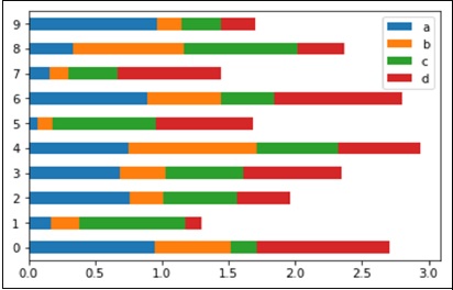
Histograms
Histograms can be plotted using the plot.hist() method. We can specify number of bins.
import pandas as pd
import numpy as np
df = pd.DataFrame({'a':np.random.randn(1000)+1,'b':np.random.randn(1000),'c':
np.random.randn(1000) - 1}, columns=['a', 'b', 'c'])
df.plot.hist(bins=20)
Its output is as follows −
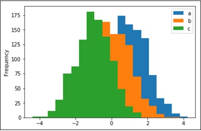
To plot different histograms for each column, use the following code −
import pandas as pd
import numpy as np
df=pd.DataFrame({'a':np.random.randn(1000)+1,'b':np.random.randn(1000),'c':
np.random.randn(1000) - 1}, columns=['a', 'b', 'c'])
df.diff.hist(bins=20)
Its output is as follows −
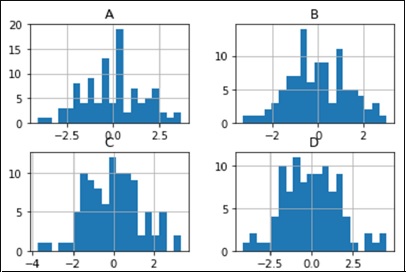
Box Plots
Boxplot can be drawn calling Series.box.plot() and DataFrame.box.plot(), or DataFrame.boxplot() to visualize the distribution of values within each column.
For instance, here is a boxplot representing five trials of 10 observations of a uniform random variable on [0,1).
import pandas as pd import numpy as np df = pd.DataFrame(np.random.rand(10, 5), columns=['A', 'B', 'C', 'D', 'E']) df.plot.box()
Its output is as follows −
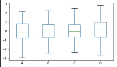
Area Plot
Area plot can be created using the Series.plot.area() or the DataFrame.plot.area() methods.
import pandas as pd import numpy as np df = pd.DataFrame(np.random.rand(10, 4), columns=['a', 'b', 'c', 'd']) df.plot.area()
Its output is as follows −
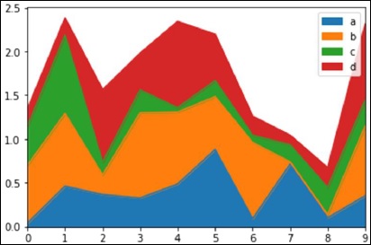
Scatter Plot
Scatter plot can be created using the DataFrame.plot.scatter() methods.
import pandas as pd import numpy as np df = pd.DataFrame(np.random.rand(50, 4), columns=['a', 'b', 'c', 'd']) df.plot.scatter(x='a', y='b')
Its output is as follows −
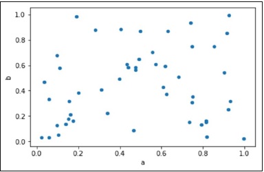
Pie Chart
Pie chart can be created using the DataFrame.plot.pie() method.
import pandas as pd import numpy as np df = pd.DataFrame(3 * np.random.rand(4), index=['a', 'b', 'c', 'd'], columns=['x']) df.plot.pie(subplots=True)
Its output is as follows −
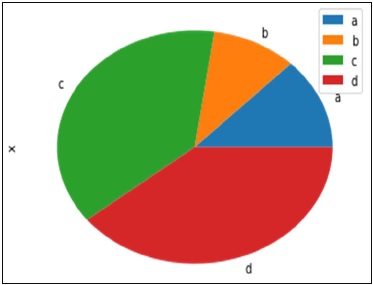
Python Pandas - IO Tools
The Pandas I/O API is a set of top level reader functions accessed like pd.read_csv() that generally return a Pandas object.
The two workhorse functions for reading text files (or the flat files) are read_csv() and read_table(). They both use the same parsing code to intelligently convert tabular data into a DataFrame object −
pandas.read_csv(filepath_or_buffer, sep=',', delimiter=None, header='infer', names=None, index_col=None, usecols=None
pandas.read_csv(filepath_or_buffer, sep='\t', delimiter=None, header='infer', names=None, index_col=None, usecols=None
Here is how the csv file data looks like −
S.No,Name,Age,City,Salary 1,Tom,28,Toronto,20000 2,Lee,32,HongKong,3000 3,Steven,43,Bay Area,8300 4,Ram,38,Hyderabad,3900
Save this data as temp.csv and conduct operations on it.
S.No,Name,Age,City,Salary 1,Tom,28,Toronto,20000 2,Lee,32,HongKong,3000 3,Steven,43,Bay Area,8300 4,Ram,38,Hyderabad,3900
Save this data as temp.csv and conduct operations on it.
read.csv
read.csv reads data from the csv files and creates a DataFrame object.
import pandas as pd
df=pd.read_csv("temp.csv")
print df
Its output is as follows −
S.No Name Age City Salary 0 1 Tom 28 Toronto 20000 1 2 Lee 32 HongKong 3000 2 3 Steven 43 Bay Area 8300 3 4 Ram 38 Hyderabad 3900
custom index
This specifies a column in the csv file to customize the index using index_col.
import pandas as pd
df=pd.read_csv("temp.csv",index_col=['S.No'])
print df
Its output is as follows −
S.No Name Age City Salary 1 Tom 28 Toronto 20000 2 Lee 32 HongKong 3000 3 Steven 43 Bay Area 8300 4 Ram 38 Hyderabad 3900
Converters
dtype of the columns can be passed as a dict.
import pandas as pd
df = pd.read_csv("temp.csv", dtype={'Salary': np.float64})
print df.dtypes
Its output is as follows −
S.No int64 Name object Age int64 City object Salary float64 dtype: object
By default, the dtype of the Salary column is int, but the result shows it as float because we have explicitly casted the type.
Thus, the data looks like float −
S.No Name Age City Salary 0 1 Tom 28 Toronto 20000.0 1 2 Lee 32 HongKong 3000.0 2 3 Steven 43 Bay Area 8300.0 3 4 Ram 38 Hyderabad 3900.0
header_names
Specify the names of the header using the names argument.
import pandas as pd
df=pd.read_csv("temp.csv", names=['a', 'b', 'c','d','e'])
print df
Its output is as follows −
a b c d e
0 S.No Name Age City Salary
1 1 Tom 28 Toronto 20000
2 2 Lee 32 HongKong 3000
3 3 Steven 43 Bay Area 8300
4 4 Ram 38 Hyderabad 3900
Observe, the header names are appended with the custom names, but the header in the file has not been eliminated. Now, we use the header argument to remove that.
If the header is in a row other than the first, pass the row number to header. This will skip the preceding rows.
import pandas as pd
df=pd.read_csv("temp.csv",names=['a','b','c','d','e'],header=0)
print df
Its output is as follows −
a b c d e
0 S.No Name Age City Salary
1 1 Tom 28 Toronto 20000
2 2 Lee 32 HongKong 3000
3 3 Steven 43 Bay Area 8300
4 4 Ram 38 Hyderabad 3900
skiprows
skiprows skips the number of rows specified.
import pandas as pd
df=pd.read_csv("temp.csv", skiprows=2)
print df
Its output is as follows −
2 Lee 32 HongKong 3000
0 3 Steven 43 Bay Area 8300
1 4 Ram 38 Hyderabad 3900
Python Pandas - Sparse Data
Sparse objects are “compressed” when any data matching a specific value (NaN / missing value, though any value can be chosen) is omitted. A special SparseIndex object tracks where data has been “sparsified”. This will make much more sense in an example. All of the standard Pandas data structures apply the to_sparse method −
import pandas as pd import numpy as np ts = pd.Series(np.random.randn(10)) ts[2:-2] = np.nan sts = ts.to_sparse() print sts
Its output is as follows −
0 -0.810497 1 -1.419954 2 NaN 3 NaN 4 NaN 5 NaN 6 NaN 7 NaN 8 0.439240 9 -1.095910 dtype: float64 BlockIndex Block locations: array([0, 8], dtype=int32) Block lengths: array([2, 2], dtype=int32)
The sparse objects exist for memory efficiency reasons.
Let us now assume you had a large NA DataFrame and execute the following code −
import pandas as pd import numpy as np df = pd.DataFrame(np.random.randn(10000, 4)) df.ix[:9998] = np.nan sdf = df.to_sparse() print sdf.density
Its output is as follows −
0.0001
Any sparse object can be converted back to the standard dense form by calling to_dense −
import pandas as pd import numpy as np ts = pd.Series(np.random.randn(10)) ts[2:-2] = np.nan sts = ts.to_sparse() print sts.to_dense()
Its output is as follows −
0 -0.810497 1 -1.419954 2 NaN 3 NaN 4 NaN 5 NaN 6 NaN 7 NaN 8 0.439240 9 -1.095910 dtype: float64
Sparse Dtypes
Sparse data should have the same dtype as its dense representation. Currently, float64, int64 and booldtypes are supported. Depending on the original dtype, fill_value default changes −
float64 − np.nan
int64 − 0
bool − False
Let us execute the following code to understand the same −
import pandas as pd import numpy as np s = pd.Series([1, np.nan, np.nan]) print s s.to_sparse() print s
Its output is as follows −
0 1.0 1 NaN 2 NaN dtype: float64 0 1.0 1 NaN 2 NaN dtype: float64
Python Pandas - Caveats & Gotchas
Caveats means warning and gotcha means an unseen problem.
Using If/Truth Statement with Pandas
Pandas follows the numpy convention of raising an error when you try to convert something to a bool. This happens in an if or when using the Boolean operations, and, or, or not. It is not clear what the result should be. Should it be True because it is not zerolength? False because there are False values? It is unclear, so instead, Pandas raises a ValueError −
import pandas as pd if pd.Series([False, True, False]): print 'I am True'
Its output is as follows −
ValueError: The truth value of a Series is ambiguous. Use a.empty, a.bool() a.item(),a.any() or a.all().
In if condition, it is unclear what to do with it. The error is suggestive of whether to use a None or any of those.
import pandas as pd
if pd.Series([False, True, False]).any():
print("I am any")
Its output is as follows −
I am any
To evaluate single-element pandas objects in a Boolean context, use the method .bool() −
import pandas as pd print pd.Series([True]).bool()
Its output is as follows −
True
Bitwise Boolean
Bitwise Boolean operators like == and != will return a Boolean series, which is almost always what is required anyways.
import pandas as pd s = pd.Series(range(5)) print s==4
Its output is as follows −
0 False 1 False 2 False 3 False 4 True dtype: bool
isin Operation
This returns a Boolean series showing whether each element in the Series is exactly contained in the passed sequence of values.
import pandas as pd
s = pd.Series(list('abc'))
s = s.isin(['a', 'c', 'e'])
print s
Its output is as follows −
0 True 1 False 2 True dtype: bool
Reindexing vs ix Gotcha
Many users will find themselves using the ix indexing capabilities as a concise means of selecting data from a Pandas object −
import pandas as pd
import numpy as np
df = pd.DataFrame(np.random.randn(6, 4), columns=['one', 'two', 'three',
'four'],index=list('abcdef'))
print df
print df.ix[['b', 'c', 'e']]
Its output is as follows −
one two three four
a -1.582025 1.335773 0.961417 -1.272084
b 1.461512 0.111372 -0.072225 0.553058
c -1.240671 0.762185 1.511936 -0.630920
d -2.380648 -0.029981 0.196489 0.531714
e 1.846746 0.148149 0.275398 -0.244559
f -1.842662 -0.933195 2.303949 0.677641
one two three four
b 1.461512 0.111372 -0.072225 0.553058
c -1.240671 0.762185 1.511936 -0.630920
e 1.846746 0.148149 0.275398 -0.244559
This is, of course, completely equivalent in this case to using the reindex method −
import pandas as pd
import numpy as np
df = pd.DataFrame(np.random.randn(6, 4), columns=['one', 'two', 'three',
'four'],index=list('abcdef'))
print df
print df.reindex(['b', 'c', 'e'])
Its output is as follows −
one two three four
a 1.639081 1.369838 0.261287 -1.662003
b -0.173359 0.242447 -0.494384 0.346882
c -0.106411 0.623568 0.282401 -0.916361
d -1.078791 -0.612607 -0.897289 -1.146893
e 0.465215 1.552873 -1.841959 0.329404
f 0.966022 -0.190077 1.324247 0.678064
one two three four
b -0.173359 0.242447 -0.494384 0.346882
c -0.106411 0.623568 0.282401 -0.916361
e 0.465215 1.552873 -1.841959 0.329404
Some might conclude that ix and reindex are 100% equivalent based on this. This is true except in the case of integer indexing. For example, the above operation can alternatively be expressed as −
import pandas as pd
import numpy as np
df = pd.DataFrame(np.random.randn(6, 4), columns=['one', 'two', 'three',
'four'],index=list('abcdef'))
print df
print df.ix[[1, 2, 4]]
print df.reindex([1, 2, 4])
Its output is as follows −
one two three four
a -1.015695 -0.553847 1.106235 -0.784460
b -0.527398 -0.518198 -0.710546 -0.512036
c -0.842803 -1.050374 0.787146 0.205147
d -1.238016 -0.749554 -0.547470 -0.029045
e -0.056788 1.063999 -0.767220 0.212476
f 1.139714 0.036159 0.201912 0.710119
one two three four
b -0.527398 -0.518198 -0.710546 -0.512036
c -0.842803 -1.050374 0.787146 0.205147
e -0.056788 1.063999 -0.767220 0.212476
one two three four
1 NaN NaN NaN NaN
2 NaN NaN NaN NaN
4 NaN NaN NaN NaN
It is important to remember that reindex is strict label indexing only. This can lead to some potentially surprising results in pathological cases where an index contains, say, both integers and strings.
Python Pandas - Comparison with SQL
Since many potential Pandas users have some familiarity with SQL, this page is meant to provide some examples of how various SQL operations can be performed using pandas.
import pandas as pd url = 'https://raw.github.com/pandasdev/ pandas/master/pandas/tests/data/tips.csv' tips=pd.read_csv(url) print tips.head()
Its output is as follows −
total_bill tip sex smoker day time size
0 16.99 1.01 Female No Sun Dinner 2
1 10.34 1.66 Male No Sun Dinner 3
2 21.01 3.50 Male No Sun Dinner 3
3 23.68 3.31 Male No Sun Dinner 2
4 24.59 3.61 Female No Sun Dinner 4
SELECT
In SQL, selection is done using a comma-separated list of columns that you select (or a * to select all columns) −
SELECT total_bill, tip, smoker, time FROM tips LIMIT 5;
With Pandas, column selection is done by passing a list of column names to your DataFrame −
tips[['total_bill', 'tip', 'smoker', 'time']].head(5)
Let’s check the full program −
import pandas as pd url = 'https://raw.github.com/pandasdev/ pandas/master/pandas/tests/data/tips.csv' tips=pd.read_csv(url) print tips[['total_bill', 'tip', 'smoker', 'time']].head(5)
Its output is as follows −
total_bill tip smoker time 0 16.99 1.01 No Dinner 1 10.34 1.66 No Dinner 2 21.01 3.50 No Dinner 3 23.68 3.31 No Dinner 4 24.59 3.61 No Dinner
Calling the DataFrame without the list of column names will display all columns (akin to SQL’s *).
WHERE
Filtering in SQL is done via a WHERE clause.
SELECT * FROM tips WHERE time = 'Dinner' LIMIT 5;
DataFrames can be filtered in multiple ways; the most intuitive of which is using Boolean indexing.
tips[tips['time'] == 'Dinner'].head(5)
Let’s check the full program −
import pandas as pd url = 'https://raw.github.com/pandasdev/ pandas/master/pandas/tests/data/tips.csv' tips=pd.read_csv(url) print tips[tips['time'] == 'Dinner'].head(5)
Its output is as follows −
total_bill tip sex smoker day time size 0 16.99 1.01 Female No Sun Dinner 2 1 10.34 1.66 Male No Sun Dinner 3 2 21.01 3.50 Male No Sun Dinner 3 3 23.68 3.31 Male No Sun Dinner 2 4 24.59 3.61 Female No Sun Dinner 4
The above statement passes a Series of True/False objects to the DataFrame, returning all rows with True.
GroupBy
This operation fetches the count of records in each group throughout a dataset. For instance, a query fetching us the number of tips left by sex −
SELECT sex, count(*) FROM tips GROUP BY sex;
The Pandas equivalent would be −
tips.groupby('sex').size()
Let’s check the full program −
import pandas as pd
url = 'https://raw.github.com/pandasdev/
pandas/master/pandas/tests/data/tips.csv'
tips=pd.read_csv(url)
print tips.groupby('sex').size()
Its output is as follows −
sex Female 87 Male 157 dtype: int64
Top N rows
SQL returns the top n rows using LIMIT −
SELECT * FROM tips LIMIT 5 ;
The Pandas equivalent would be −
tips.head(5)
Let’s check the full example −
import pandas as pd url = 'https://raw.github.com/pandas-dev/pandas/master/pandas/tests/data/tips.csv' tips=pd.read_csv(url) tips = tips[['smoker', 'day', 'time']].head(5) print tips
Its output is as follows −
smoker day time 0 No Sun Dinner 1 No Sun Dinner 2 No Sun Dinner 3 No Sun Dinner 4 No Sun Dinner
These are the few basic operations we compared are, which we learnt, in the previous chapters of the Pandas Library.