Python Deep Learning - Quick Guide

---

---

Python Deep Learning - Introduction

Deep structured learning or hierarchical learning or deep learning in short is part of the family of machine learning methods which are themselves a subset of the broader field of Artificial Intelligence.

Deep learning is a class of machine learning algorithms that use several layers of nonlinear processing units for feature extraction and transformation. Each successive layer uses the output from the previous layer as input.

Deep neural networks, deep belief networks and recurrent neural networks have been applied to fields such as computer vision, speech recognition, natural language processing, audio recognition, social network filtering, machine translation, and bioinformatics where they produced results comparable to and in some cases better than human experts have.

Deep Learning Algorithms and Networks −

• are based on the unsupervised learning of multiple levels of features or representations of the data. Higher-level features are derived from lower level features to form a hierarchical representation.

• use some form of gradient descent for training.

Python Deep Learning - Environment

In this chapter, we will learn about the environment set up for Python Deep Learning. We have to install the following software for making deep learning algorithms.

• Python 2.7+
• Scipy with Numpy
• Matplotlib
• Theano
• Keras
• TensorFlow

It is strongly recommend that Python, NumPy, SciPy, and Matplotlib are installed through the Anaconda distribution. It comes with all of those packages.

We need to ensure that the different types of software are installed properly.

Let us go to our command line program and type in the following command −

$ python
Python 3.6.3 |Anaconda custom (32-bit)| (default, Oct 13 2017, 14:21:34)
[GCC 7.2.0] on linux

Next, we can import the required libraries and print their versions −

import numpy
print numpy.__version__

Output

1.14.2

Installation of Theano, TensorFlow and Keras

Before we begin with the installation of the packages − Theano, TensorFlow and Keras, we need to confirm if the pip is installed. The package management system in Anaconda is called the pip.

To confirm the installation of pip, type the following in the command line −

$ pip

Once the installation of pip is confirmed, we can install TensorFlow and Keras by executing the following command −

$pip install theano
$pip install tensorflow
$pip install keras

Confirm the installation of Theano by executing the following line of code −

$python –c “import theano: print (theano.__version__)”

Output

1.0.1

Confirm the installation of Tensorflow by executing the following line of code −

$python –c “import tensorflow: print tensorflow.__version__”

Output

1.7.0

Confirm the installation of Keras by executing the following line of code −

$python –c “import keras: print keras.__version__”
Using TensorFlow backend

Output

2.1.5

Python Deep Basic Machine Learning

Artificial Intelligence (AI) is any code, algorithm or technique that enables a computer to mimic human cognitive behaviour or intelligence. Machine Learning (ML) is a subset of AI that uses statistical methods to enable machines to learn and improve with experience. Deep Learning is a subset of Machine Learning, which makes the computation of multi-layer neural networks feasible. Machine Learning is seen as shallow learning while Deep Learning is seen as hierarchical learning with abstraction.

Machine learning deals with a wide range of concepts. The concepts are listed below −

• supervised
• unsupervised
• reinforcement learning
• linear regression
• cost functions
• overfitting
• under-fitting
• hyper-parameter, etc.

In supervised learning, we learn to predict values from labelled data. One ML technique that helps here is classification, where target values are discrete values; for example,cats and dogs. Another technique in machine learning that could come of help is regression. Regression works onthe target values. The target values are continuous values; for example, the stock market data can be analysed using Regression.

In unsupervised learning, we make inferences from the input data that is not labelled or structured. If we have a million medical records and we have to make sense of it, find the underlying structure, outliers or detect anomalies, we use clustering technique to divide data into broad clusters.

Data sets are divided into training sets, testing sets, validation sets and so on.

A breakthrough in 2012 brought the concept of Deep Learning into prominence. An algorithm classified 1 million images into 1000 categories successfully using 2 GPUs and latest technologies like Big Data.

Relating Deep Learning and Traditional Machine Learning

One of the major challenges encountered in traditional machine learning models is a process called feature extraction. The programmer needs to be specific and tell the computer the features to be looked out for. These features will help in making decisions.

Entering raw data into the algorithm rarely works, so feature extraction is a critical part of the traditional machine learning workflow.

This places a huge responsibility on the programmer, and the algorithm's efficiency relies heavily on how inventive the programmer is. For complex problems such as object recognition or handwriting recognition, this is a huge issue.

Deep learning, with the ability to learn multiple layers of representation, is one of the few methods that has help us with automatic feature extraction. The lower layers can be assumed to be performing automatic feature extraction, requiring little or no guidance from the programmer.

Artificial Neural Networks

The Artificial Neural Network, or just neural network for short, is not a new idea. It has been around for about 80 years.

It was not until 2011, when Deep Neural Networks became popular with the use of new techniques, huge dataset availability, and powerful computers.

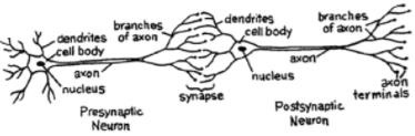
A neural network mimics a neuron, which has dendrites, a nucleus, axon, and terminal axon.

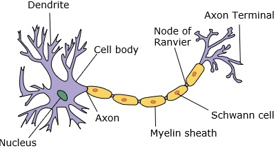
For a network, we need two neurons. These neurons transfer information via synapse between the dendrites of one and the terminal axon of another.

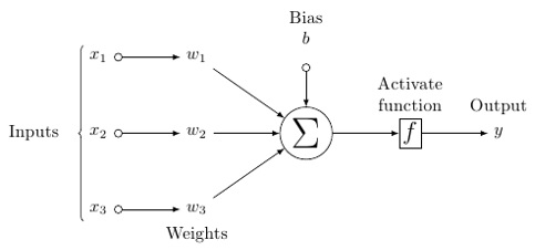
A probable model of an artificial neuron looks like this −

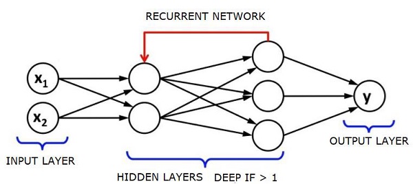
A neural network will look like as shown below −

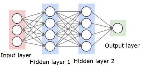
The circles are neurons or nodes, with their functions on the data and the lines/edges connecting them are the weights/information being passed along.

Each column is a layer. The first layer of your data is the input layer. Then, all the layers between the input layer and the output layer are the hidden layers.

If you have one or a few hidden layers, then you have a shallow neural network. If you have many hidden layers, then you have a deep neural network.

In this model, you have input data, you weight it, and pass it through the function in the neuron that is called threshold function or activation function.

Basically, it is the sum of all of the values after comparing it with a certain value. If you fire a signal, then the result is (1) out, or nothing is fired out, then (0). That is then weighted and passed along to the next neuron, and the same sort of function is run.

We can have a sigmoid (s-shape) function as the activation function.

As for the weights, they are just random to start, and they are unique per input into the node/neuron.

In a typical "feed forward", the most basic type of neural network, you have your information pass straight through the network you created, and you compare the output to what you hoped the output would have been using your sample data.

From here, you need to adjust the weights to help you get your output to match your desired output.

The act of sending data straight through a neural network is called a feed forward neural network.

Our data goes from input, to the layers, in order, then to the output.

When we go backwards and begin adjusting weights to minimize loss/cost, this is called back propagation.

This is an optimization problem. With the neural network, in real practice, we have to deal with hundreds of thousands of variables, or millions, or more.

The first solution was to use stochastic gradient descent as optimization method. Now, there are options like AdaGrad, Adam Optimizer and so on. Either way, this is a massive computational operation. That is why Neural Networks were mostly left on the shelf for over half a century. It was only very recently that we even had the power and architecture in our machines to even consider doing these operations, and the properly sized datasets to match.

For simple classification tasks, the neural network is relatively close in performance to other simple algorithms like K Nearest Neighbors. The real utility of neural networks is realized when we have much larger data, and much more complex questions, both of which outperform other machine learning models.

Deep Neural Networks

A deep neural network (DNN) is an ANN with multiple hidden layers between the input and output layers. Similar to shallow ANNs, DNNs can model complex non-linear relationships.

The main purpose of a neural network is to receive a set of inputs, perform progressively complex calculations on them, and give output to solve real world problems like classification. We restrict ourselves to feed forward neural networks.

We have an input, an output, and a flow of sequential data in a deep network.

Neural networks are widely used in supervised learning and reinforcement learning problems. These networks are based on a set of layers connected to each other.

In deep learning, the number of hidden layers, mostly non-linear, can be large; say about 1000 layers.

DL models produce much better results than normal ML networks.

We mostly use the gradient descent method for optimizing the network and minimising the loss function.

We can use the Imagenet, a repository of millions of digital images to classify a dataset into categories like cats and dogs. DL nets are increasingly used for dynamic images apart from static ones and for time series and text analysis.

Training the data sets forms an important part of Deep Learning models. In addition, Backpropagation is the main algorithm in training DL models.

DL deals with training large neural networks with complex input output transformations.

One example of DL is the mapping of a photo to the name of the person(s) in photo as they do on social networks and describing a picture with a phrase is another recent application of DL.

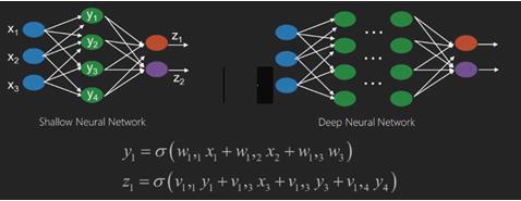
Neural networks are functions that have inputs like x1,x2,x3…that are transformed to outputs like z1,z2,z3 and so on in two (shallow networks) or several intermediate operations also called layers (deep networks).

The weights and biases change from layer to layer. ‘w’ and ‘v’ are the weights or synapses of layers of the neural networks.

The best use case of deep learning is the supervised learning problem.Here,we have large set of data inputs with a desired set of outputs.

Here we apply back propagation algorithm to get correct output prediction.

The most basic data set of deep learning is the MNIST, a dataset of handwritten digits.

We can train deep a Convolutional Neural Network with Keras to classify images of handwritten digits from this dataset.

The firing or activation of a neural net classifier produces a score. For example,to classify patients as sick and healthy,we consider parameters such as height, weight and body temperature, blood pressure etc.

A high score means patient is sick and a low score means he is healthy.

Each node in output and hidden layers has its own classifiers. The input layer takes inputs and passes on its scores to the next hidden layer for further activation and this goes on till the output is reached.

This progress from input to output from left to right in the forward direction is called forward propagation.

Credit assignment path (CAP) in a neural network is the series of transformations starting from the input to the output. CAPs elaborate probable causal connections between the input and the output.

CAP depth for a given feed forward neural network or the CAP depth is the number of hidden layers plus one as the output layer is included. For recurrent neural networks, where a signal may propagate through a layer several times, the CAP depth can be potentially limitless.

Deep Nets and Shallow Nets

There is no clear threshold of depth that divides shallow learning from deep learning; but it is mostly agreed that for deep learning which has multiple non-linear layers, CAP must be greater than two.

Basic node in a neural net is a perception mimicking a neuron in a biological neural network. Then we have multi-layered Perception or MLP. Each set of inputs is modified by a set of weights and biases; each edge has a unique weight and each node has a unique bias.

The prediction accuracy of a neural net depends on its weights and biases.

The process of improving the accuracy of neural network is called training. The output from a forward prop net is compared to that value which is known to be correct.

The cost function or the loss function is the difference between the generated output and the actual output.

The point of training is to make the cost of training as small as possible across millions of training examples.To do this, the network tweaks the weights and biases until the prediction matches the correct output.

Once trained well, a neural net has the potential to make an accurate prediction every time.

When the pattern gets complex and you want your computer to recognise them, you have to go for neural networks.In such complex pattern scenarios, neural network outperformsall other competing algorithms.

There are now GPUs that can train them faster than ever before. Deep neural networks are already revolutionizing the field of AI

Computers have proved to be good at performing repetitive calculations and following detailed instructions but have been not so good at recognising complex patterns.

If there is the problem of recognition of simple patterns, a support vector machine (svm) or a logistic regression classifier can do the job well, but as the complexity of patternincreases, there is no way but to go for deep neural networks.

Therefore, for complex patterns like a human face, shallow neural networks fail and have no alternative but to go for deep neural networks with more layers. The deep nets are able to do their job by breaking down the complex patterns into simpler ones. For example, human face; adeep net would use edges to detect parts like lips, nose, eyes, ears and so on and then re-combine these together to form a human face

The accuracy of correct prediction has become so accurate that recently at a Google Pattern Recognition Challenge, a deep net beat a human.

This idea of a web of layered perceptrons has been around for some time; in this area, deep nets mimic the human brain. But one downside to this is that they take long time to train, a hardware constraint

However recent high performance GPUs have been able to train such deep nets under a week; while fast cpus could have taken weeks or perhaps months to do the same.

Choosing a Deep Net

How to choose a deep net? We have to decide if we are building a classifier or if we are trying to find patterns in the data and if we are going to use unsupervised learning. To extract patterns from a set of unlabelled data, we use a Restricted Boltzman machine or an Auto encoder.

Consider the following points while choosing a deep net −

• For text processing, sentiment analysis, parsing and name entity recognition, we use a recurrent net or recursive neural tensor network or RNTN;

• For any language model that operates at character level, we use the recurrent net.

• For image recognition, we use deep belief network DBN or convolutional network.

• For object recognition, we use a RNTN or a convolutional network.

• For speech recognition, we use recurrent net.

In general, deep belief networks and multilayer perceptrons with rectified linear units or RELU are both good choices for classification.

For time series analysis, it is always recommended to use recurrent net.

Neural nets have been around for more than 50 years; but only now they have risen into prominence. The reason is that they are hard to train; when we try to train them with a method called back propagation, we run into a problem called vanishing or exploding gradients.When that happens, training takes a longer time and accuracy takes a back-seat. When training a data set, we are constantly calculating the cost function, which is the difference between predicted output and the actual output from a set of labelled training data.The cost function is then minimized by adjusting the weights and biases values until the lowest value is obtained. The training process uses a gradient, which is the rate at which the cost will change with respect to change in weight or bias values.

Restricted Boltzman Networks or Autoencoders - RBNs

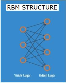
In 2006, a breakthrough was achieved in tackling the issue of vanishing gradients. Geoff Hinton devised a novel strategy that led to the development of Restricted Boltzman Machine - RBM, a shallow two layer net.

The first layer is the visible layer and the second layer is the hidden layer. Each node in the visible layer is connected to every node in the hidden layer. The network is known as restricted as no two layers within the same layer are allowed to share a connection.

Autoencoders are networks that encode input data as vectors. They create a hidden, or compressed, representation of the raw data. The vectors are useful in dimensionality reduction; the vector compresses the raw data into smaller number of essential dimensions. Autoencoders are paired with decoders, which allows the reconstruction of input data based on its hidden representation.

RBM is the mathematical equivalent of a two-way translator. A forward pass takes inputs and translates them into a set of numbers that encodes the inputs. A backward pass meanwhile takes this set of numbers and translates them back into reconstructed inputs. A well-trained net performs back prop with a high degree of accuracy.

In either steps, the weights and the biases have a critical role; they help the RBM in decoding the interrelationships between the inputs and in deciding which inputs are essential in detecting patterns. Through forward and backward passes, the RBM is trained to re-construct the input with different weights and biases until the input and there-construction are as close as possible. An interesting aspect of RBM is that data need not be labelled. This turns out to be very important for real world data sets like photos, videos, voices and sensor data, all of which tend to be unlabelled. Instead of manually labelling data by humans, RBM automatically sorts through data; by properly adjusting the weights and biases, an RBM is able to extract important features and reconstruct the input. RBM is a part of family of feature extractor neural nets, which are designed to recognize inherent patterns in data. These are also called auto-encoders because they have to encode their own structure.

Deep Belief Networks - DBNs

Deep belief networks (DBNs) are formed by combining RBMs and introducing a clever training method. We have a new model that finally solves the problem of vanishing gradient. Geoff Hinton invented the RBMs and also Deep Belief Nets as alternative to back propagation.

A DBN is similar in structure to a MLP (Multi-layer perceptron), but very different when it comes to training. it is the training that enables DBNs to outperform their shallow counterparts

A DBN can be visualized as a stack of RBMs where the hidden layer of one RBM is the visible layer of the RBM above it. The first RBM is trained to reconstruct its input as accurately as possible.

The hidden layer of the first RBM is taken as the visible layer of the second RBM and the second RBM is trained using the outputs from the first RBM. This process is iterated till every layer in the network is trained.

In a DBN, each RBM learns the entire input. A DBN works globally by fine-tuning the entire input in succession as the model slowly improves like a camera lens slowly focussing a picture. A stack of RBMs outperforms a single RBM as a multi-layer perceptron MLP outperforms a single perceptron.

At this stage, the RBMs have detected inherent patterns in the data but without any names or label. To finish training of the DBN, we have to introduce labels to the patterns and fine tune the net with supervised learning.

We need a very small set of labelled samples so that the features and patterns can be associated with a name. This small-labelled set of data is used for training. This set of labelled data can be very small when compared to the original data set.

The weights and biases are altered slightly, resulting in a small change in the net's perception of the patterns and often a small increase in the total accuracy.

The training can also be completed in a reasonable amount of time by using GPUs giving very accurate results as compared to shallow nets and we see a solution to vanishing gradient problem too.

Generative Adversarial Networks - GANs

Generative adversarial networks are deep neural nets comprising two nets, pitted one against the other, thus the “adversarial” name.

GANs were introduced in a paper published by researchers at the University of Montreal in 2014. Facebook’s AI expert Yann LeCun, referring to GANs, called adversarial training “the most interesting idea in the last 10 years in ML.”

GANs’ potential is huge, as the network-scan learn to mimic any distribution of data. GANs can be taught to create parallel worlds strikingly similar to our own in any domain: images, music, speech, prose. They are robot artists in a way, and their output is quite impressive.

In a GAN, one neural network, known as the generator, generates new data instances, while the other, the discriminator, evaluates them for authenticity.

Let us say we are trying to generate hand-written numerals like those found in the MNIST dataset, which is taken from the real world. The work of the discriminator, when shown an instance from the true MNIST dataset, is to recognize them as authentic.

Now consider the following steps of the GAN −

• The generator network takes input in the form of random numbers and returns an image.

• This generated image is given as input to the discriminator network along with a stream of images taken from the actual dataset.

• The discriminator takes in both real and fake images and returns probabilities, a number between 0 and 1, with 1 representing a prediction of authenticity and 0 representing fake.

• So you have a double feedback loop −

  • The discriminator is in a feedback loop with the ground truth of the images, which we know.

  • The generator is in a feedback loop with the discriminator.

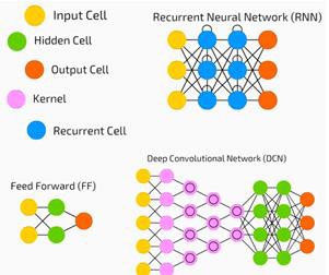
Recurrent Neural Networks - RNNs

RNNSare neural networks in which data can flow in any direction. These networks are used for applications such as language modelling or Natural Language Processing (NLP).

The basic concept underlying RNNs is to utilize sequential information. In a normal neural network it is assumed that all inputs and outputs are independent of each other. If we want to predict the next word in a sentence we have to know which words came before it.

RNNs are called recurrent as they repeat the same task for every element of a sequence, with the output being based on the previous computations. RNNs thus can be said to have a “memory” that captures information about what has been previously calculated. In theory, RNNs can use information in very long sequences, but in reality, they can look back only a few steps.

Long short-term memory networks (LSTMs) are most commonly used RNNs.

Together with convolutional Neural Networks, RNNs have been used as part of a model to generate descriptions for unlabelled images. It is quite amazing how well this seems to work.

Convolutional Deep Neural Networks - CNNs

If we increase the number of layers in a neural network to make it deeper, it increases the complexity of the network and allows us to model functions that are more complicated. However, the number of weights and biases will exponentially increase. As a matter of fact, learning such difficult problems can become impossible for normal neural networks. This leads to a solution, the convolutional neural networks.

CNNs are extensively used in computer vision; have been applied also in acoustic modelling for automatic speech recognition.

The idea behind convolutional neural networks is the idea of a “moving filter” which passes through the image. This moving filter, or convolution, applies to a certain neighbourhood of nodes which for example may be pixels, where the filter applied is 0.5 x the node value −

Noted researcher Yann LeCun pioneered convolutional neural networks. Facebook as facial recognition software uses these nets. CNN have been the go to solution for machine vision projects. There are many layers to a convolutional network. In Imagenet challenge, a machine was able to beat a human at object recognition in 2015.

In a nutshell, Convolutional Neural Networks (CNNs) are multi-layer neural networks. The layers are sometimes up to 17 or more and assume the input data to be images.

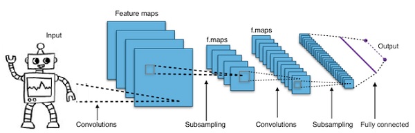
CNNs drastically reduce the number of parameters that need to be tuned. So, CNNs efficiently handle the high dimensionality of raw images.

Python Deep Learning - Fundamentals

In this chapter, we will look into the fundamentals of Python Deep Learning.

Deep learning models/algorithms

Let us now learn about the different deep learning models/ algorithms.

Some of the popular models within deep learning are as follows −

• Convolutional neural networks
• Recurrent neural networks
• Deep belief networks
• Generative adversarial networks
• Auto-encoders and so on

The inputs and outputs are represented as vectors or tensors. For example, a neural network may have the inputs where individual pixel RGB values in an image are represented as vectors.

The layers of neurons that lie between the input layer and the output layer are called hidden layers. This is where most of the work happens when the neural net tries to solve problems. Taking a closer look at the hidden layers can reveal a lot about the features the network has learned to extract from the data.

Different architectures of neural networks are formed by choosing which neurons to connect to the other neurons in the next layer.

Pseudocode for calculating output

Following is the pseudocode for calculating output of Forward-propagating Neural Network −

• # node[] := array of topologically sorted nodes
• # An edge from a to b means a is to the left of b
• # If the Neural Network has R inputs and S outputs,
• # then first R nodes are input nodes and last S nodes are output nodes.
• # incoming[x] := nodes connected to node x
• # weight[x] := weights of incoming edges to x

For each neuron x, from left to right −

• if x <= R: do nothing # its an input node
• inputs[x] = [output[i] for i in incoming[x]]
• weighted_sum = dot_product(weights[x], inputs[x])
• output[x] = Activation_function(weighted_sum)

Training a Neural Network

We will now learn how to train a neural network. We will also learn back propagation algorithm and backward pass in Python Deep Learning.

We have to find the optimal values of the weights of a neural network to get the desired output. To train a neural network, we use the iterative gradient descent method. We start initially with random initialization of the weights. After random initialization, we make predictions on some subset of the data with forward-propagation process, compute the corresponding cost function C, and update each weight w by an amount proportional to dC/dw, i.e., the derivative of the cost functions w.r.t. the weight. The proportionality constant is known as the learning rate.

The gradients can be calculated efficiently using the back-propagation algorithm. The key observation of backward propagation or backward prop is that because of the chain rule of differentiation, the gradient at each neuron in the neural network can be calculated using the gradient at the neurons, it has outgoing edges to. Hence, we calculate the gradients backwards, i.e., first calculate the gradients of the output layer, then the top-most hidden layer, followed by the preceding hidden layer, and so on, ending at the input layer.

The back-propagation algorithm is implemented mostly using the idea of a computational graph, where each neuron is expanded to many nodes in the computational graph and performs a simple mathematical operation like addition, multiplication. The computational graph does not have any weights on the edges; all weights are assigned to the nodes, so the weights become their own nodes. The backward propagation algorithm is then run on the computational graph. Once the calculation is complete, only the gradients of the weight nodes are required for update. The rest of the gradients can be discarded.

Gradient Descent Optimization Technique

One commonly used optimization function that adjusts weights according to the error they caused is called the “gradient descent.”

Gradient is another name for slope, and slope, on an x-y graph, represents how two variables are related to each other: the rise over the run, the change in distance over the change in time, etc. In this case, the slope is the ratio between the network’s error and a single weight; i.e., how does the error change as the weight is varied.

To put it more precisely, we want to find which weight produces the least error. We want to find the weight that correctly represents the signals contained in the input data, and translates them to a correct classification.

As a neural network learns, it slowly adjusts many weights so that they can map signal to meaning correctly. The ratio between network Error and each of those weights is a derivative, dE/dw that calculates the extent to which a slight change in a weight causes a slight change in the error.

Each weight is just one factor in a deep network that involves many transforms; the signal of the weight passes through activations and sums over several layers, so we use the chain rule of calculus to work back through the network activations and outputs.This leads us to the weight in question, and its relationship to overall error.

Given two variables, error and weight, are mediated by a third variable, activation, through which the weight is passed. We can calculate how a change in weight affects a change in error by first calculating how a change in activation affects a change in Error, and how a change in weight affects a change in activation.

The basic idea in deep learning is nothing more than that: adjusting a model’s weights in response to the error it produces, until you cannot reduce the error any more.

The deep net trains slowly if the gradient value is small and fast if the value is high. Any inaccuracies in training leads to inaccurate outputs. The process of training the nets from the output back to the input is called back propagation or back prop. We know that forward propagation starts with the input and works forward. Back prop does the reverse/opposite calculating the gradient from right to left.

Each time we calculate a gradient, we use all the previous gradients up to that point.

Let us start at a node in the output layer. The edge uses the gradient at that node. As we go back into the hidden layers, it gets more complex. The product of two numbers between 0 and 1 gives youa smaller number. The gradient value keeps getting smaller and as a result back prop takes a lot of time to train and accuracy suffers.

Challenges in Deep Learning Algorithms

There are certain challenges for both shallow neural networks and deep neural networks, like overfitting and computation time. DNNs are affected by overfitting because the use of added layers of abstraction which allow them to model rare dependencies in the training data.

Regularization methods such as drop out, early stopping, data augmentation, transfer learning are applied during training to combat overfitting. Drop out regularization randomly omits units from the hidden layers during training which helps in avoiding rare dependencies. DNNs take into consideration several training parameters such as the size, i.e., the number of layers and the number of units per layer, the learning rate and initial weights. Finding optimal parameters is not always practical due to the high cost in time and computational resources. Several hacks such as batching can speed up computation. The large processing power of GPUs has significantly helped the training process, as the matrix and vector computations required are well-executed on the GPUs.

Dropout

Dropout is a popular regularization technique for neural networks. Deep neural networks are particularly prone to overfitting.

Let us now see what dropout is and how it works.

In the words of Geoffrey Hinton, one of the pioneers of Deep Learning, ‘If you have a deep neural net and it's not overfitting, you should probably be using a bigger one and using dropout’.

Dropout is a technique where during each iteration of gradient descent, we drop a set of randomly selected nodes. This means that we ignore some nodes randomly as if they do not exist.

Each neuron is kept with a probability of q and dropped randomly with probability 1-q. The value q may be different for each layer in the neural network. A value of 0.5 for the hidden layers, and 0 for input layer works well on a wide range of tasks.

During evaluation and prediction, no dropout is used. The output of each neuron is multiplied by q so that the input to the next layer has the same expected value.

The idea behind Dropout is as follows − In a neural network without dropout regularization, neurons develop co-dependency amongst each other that leads to overfitting.

Implementation trick

Dropout is implemented in libraries such as TensorFlow and Pytorch by keeping the output of the randomly selected neurons as 0. That is, though the neuron exists, its output is overwritten as 0.

Early Stopping

We train neural networks using an iterative algorithm called gradient descent.

The idea behind early stopping is intuitive; we stop training when the error starts to increase. Here, by error, we mean the error measured on validation data, which is the part of training data used for tuning hyper-parameters. In this case, the hyper-parameter is the stop criteria.

Data Augmentation

The process where we increase the quantum of data we have or augment it by using existing data and applying some transformations on it. The exact transformations used depend on the task we intend to achieve. Moreover, the transformations that help the neural net depend on its architecture.

For instance, in many computer vision tasks such as object classification, an effective data augmentation technique is adding new data points that are cropped or translated versions of original data.

When a computer accepts an image as an input, it takes in an array of pixel values. Let us say that the whole image is shifted left by 15 pixels. We apply many different shifts in different directions, resulting in an augmented dataset many times the size of the original dataset.

Transfer Learning

The process of taking a pre-trained model and “fine-tuning” the model with our own dataset is called transfer learning. There are several ways to do this.A few ways are described below −

• We train the pre-trained model on a large dataset. Then, we remove the last layer of the network and replace it with a new layer with random weights.

• We then freeze the weights of all the other layers and train the network normally. Here freezing the layers is not changing the weights during gradient descent or optimization.

The concept behind this is that the pre-trained model will act as a feature extractor, and only the last layer will be trained on the current task.

Computational Graphs

Backpropagation is implemented in deep learning frameworks like Tensorflow, Torch, Theano, etc., by using computational graphs. More significantly, understanding back propagation on computational graphs combines several different algorithms and its variations such as backprop through time and backprop with shared weights. Once everything is converted into a computational graph, they are still the same algorithm − just back propagation on computational graphs.

What is Computational Graph

A computational graph is defined as a directed graph where the nodes correspond to mathematical operations. Computational graphs are a way of expressing and evaluating a mathematical expression.

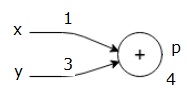
For example, here is a simple mathematical equation −

$$p = x+y$$

We can draw a computational graph of the above equation as follows.

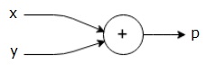
The above computational graph has an addition node (node with "+" sign) with two input variables x and y and one output q.

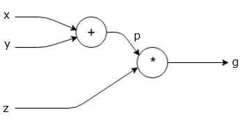
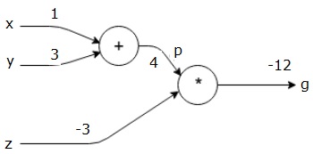
Let us take another example, slightly more complex. We have the following equation.

$$g = \left (x+y \right ) \ast z $$

The above equation is represented by the following computational graph.

Computational Graphs and Backpropagation

Computational graphs and backpropagation, both are important core concepts in deep learning for training neural networks.

Forward Pass

Forward pass is the procedure for evaluating the value of the mathematical expression represented by computational graphs. Doing forward pass means we are passing the value from variables in forward direction from the left (input) to the right where the output is.

Let us consider an example by giving some value to all of the inputs. Suppose, the following values are given to all of the inputs.

$$x=1, y=3, z=−3$$

By giving these values to the inputs, we can perform forward pass and get the following values for the outputs on each node.

First, we use the value of x = 1 and y = 3, to get p = 4.

Then we use p = 4 and z = -3 to get g = -12. We go from left to right, forwards.

Objectives of Backward Pass

In the backward pass, our intention is to compute the gradients for each input with respect to the final output. These gradients are essential for training the neural network using gradient descent.

For example, we desire the following gradients.

Desired gradients

$$\frac{\partial x}{\partial f}, \frac{\partial y}{\partial f}, \frac{\partial z}{\partial f}$$

Backward pass (backpropagation)

We start the backward pass by finding the derivative of the final output with respect to the final output (itself!). Thus, it will result in the identity derivation and the value is equal to one.

$$\frac{\partial g}{\partial g} = 1$$

Our computational graph now looks as shown below −

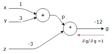
Next, we will do the backward pass through the "*" operation. We will calculate the gradients at p and z. Since g = p*z, we know that −

$$\frac{\partial g}{\partial z} = p$$

$$\frac{\partial g}{\partial p} = z$$

We already know the values of z and p from the forward pass. Hence, we get −

$$\frac{\partial g}{\partial z} = p = 4$$

and

$$\frac{\partial g}{\partial p} = z = -3$$

We want to calculate the gradients at x and y −

$$\frac{\partial g}{\partial x}, \frac{\partial g}{\partial y}$$

However, we want to do this efficiently (although x and g are only two hops away in this graph, imagine them being really far from each other). To calculate these values efficiently, we will use the chain rule of differentiation. From chain rule, we have −

$$\frac{\partial g}{\partial x}=\frac{\partial g}{\partial p}\ast \frac{\partial p}{\partial x}$$

$$\frac{\partial g}{\partial y}=\frac{\partial g}{\partial p}\ast \frac{\partial p}{\partial y}$$

But we already know the dg/dp = -3, dp/dx and dp/dy are easy since p directly depends on x and y. We have −

$$p=x+y\Rightarrow \frac{\partial x}{\partial p} = 1, \frac{\partial y}{\partial p} = 1$$

Hence, we get −

$$\frac{\partial g} {\partial f} = \frac{\partial g} {\partial p}\ast \frac{\partial p} {\partial x} = \left ( -3 \right ).1 = -3$$

In addition, for the input y −

$$\frac{\partial g} {\partial y} = \frac{\partial g} {\partial p}\ast \frac{\partial p} {\partial y} = \left ( -3 \right ).1 = -3$$

The main reason for doing this backwards is that when we had to calculate the gradient at x, we only used already computed values, and dq/dx (derivative of node output with respect to the same node's input). We used local information to compute a global value.

Steps for training a neural network

Follow these steps to train a neural network −

• For data point x in dataset,we do forward pass with x as input, and calculate the cost c as output.

• We do backward pass starting at c, and calculate gradients for all nodes in the graph. This includes nodes that represent the neural network weights.

• We then update the weights by doing W = W - learning rate * gradients.

• We repeat this process until stop criteria is met.

Python Deep Learning - Applications

Deep learning has produced good results for a few applications such as computer vision, language translation, image captioning, audio transcription, molecular biology, speech recognition, natural language processing, self-driving cars, brain tumour detection, real-time speech translation, music composition, automatic game playing and so on.

Deep learning is the next big leap after machine learning with a more advanced implementation. Currently, it is heading towards becoming an industry standard bringing a strong promise of being a game changer when dealing with raw unstructured data.

Deep learning is currently one of the best solution providers fora wide range of real-world problems. Developers are building AI programs that, instead of using previously given rules, learn from examples to solve complicated tasks. With deep learning being used by many data scientists, deeper neural networks are delivering results that are ever more accurate.

The idea is to develop deep neural networks by increasing the number of training layers for each network; machine learns more about the data until it is as accurate as possible. Developers can use deep learning techniques to implement complex machine learning tasks, and train AI networks to have high levels of perceptual recognition.

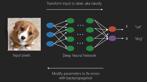
Deep learning finds its popularity in Computer vision. Here one of the tasks achieved is image classification where given input images are classified as cat, dog, etc. or as a class or label that best describe the image. We as humans learn how to do this task very early in our lives and have these skills of quickly recognizing patterns, generalizing from prior knowledge, and adapting to different image environments.

Libraries and Frameworks

In this chapter, we will relate deep learning to the different libraries and frameworks.

Deep learning and Theano

If we want to start coding a deep neural network, it is better we have an idea how different frameworks like Theano, TensorFlow, Keras, PyTorch etc work.

Theano is python library which provides a set of functions for building deep nets that train quickly on our machine.

Theano was developed at the University of Montreal, Canada under the leadership of Yoshua Bengio a deep net pioneer.

Theano lets us define and evaluate mathematical expressions with vectors and matrices which are rectangular arrays of numbers.

Technically speaking, both neural nets and input data can be represented as matrices and all standard net operations can be redefined as matrix operations. This is important since computers can carry out matrix operations very quickly.

We can process multiple matrix values in parallel and if we build a neural net with this underlying structure, we can use a single machine with a GPU to train enormous nets in a reasonable time window.

However if we use Theano, we have to build the deep net from ground up. The library does not provide complete functionality for creating a specific type of deep net.

Instead, we have to code every aspect of the deep net like the model, the layers, the activation, the training method and any special methods to stop overfitting.

The good news however is that Theano allows the building our implementation over a top of vectorized functions providing us with a highly optimized solution.

There are many other libraries that extend the functionality of Theano. TensorFlow and Keras can be used with Theano as backend.

Deep Learning with TensorFlow

Googles TensorFlow is a python library. This library is a great choice for building commercial grade deep learning applications.

TensorFlow grew out of another library DistBelief V2 that was a part of Google Brain Project. This library aims to extend the portability of machine learning so that research models could be applied to commercial-grade applications.

Much like the Theano library, TensorFlow is based on computational graphs where a node represents persistent data or math operation and edges represent the flow of data between nodes, which is a multidimensional array or tensor; hence the name TensorFlow

The output from an operation or a set of operations is fed as input into the next.

Even though TensorFlow was designed for neural networks, it works well for other nets where computation can be modelled as data flow graph.

TensorFlow also uses several features from Theano such as common and sub-expression elimination, auto differentiation, shared and symbolic variables.

Different types of deep nets can be built using TensorFlow like convolutional nets, Autoencoders, RNTN, RNN, RBM, DBM/MLP and so on.

However, there is no support for hyper parameter configuration in TensorFlow.For this functionality, we can use Keras.

Deep Learning and Keras

Keras is a powerful easy-to-use Python library for developing and evaluating deep learning models.

It has a minimalist design that allows us to build a net layer by layer; train it, and run it.

It wraps the efficient numerical computation libraries Theano and TensorFlow and allows us to define and train neural network models in a few short lines of code.

It is a high-level neural network API, helping to make wide use of deep learning and artificial intelligence. It runs on top of a number of lower-level libraries including TensorFlow, Theano,and so on. Keras code is portable; we can implement a neural network in Keras using Theano or TensorFlow as a back ended without any changes in code.

Python Deep Learning - Implementations

In this implementation of Deep learning, our objective is to predict the customer attrition or churning data for a certain bank - which customers are likely to leave this bank service. The Dataset used is relatively small and contains 10000 rows with 14 columns. We are using Anaconda distribution, and frameworks like Theano, TensorFlow and Keras. Keras is built on top of Tensorflow and Theano which function as its backends.

# Artificial Neural Network
# Installing Theano
pip install --upgrade theano

# Installing Tensorflow
pip install –upgrade tensorflow

# Installing Keras
pip install --upgrade keras

Step 1: Data preprocessing

In[]:

# Importing the libraries
   import numpy as np
   import matplotlib.pyplot as plt
   import pandas as pd
 
# Importing the database
   dataset = pd.read_csv('Churn_Modelling.csv')

Step 2

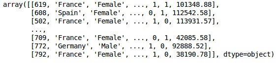
We create matrices of the features of dataset and the target variable, which is column 14, labeled as “Exited”.

The initial look of data is as shown below −

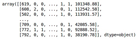
In[]:
X = dataset.iloc[:, 3:13].values
Y = dataset.iloc[:, 13].values
X

Output

Step 3

Y

Output

array([1, 0, 1, ..., 1, 1, 0], dtype = int64)

Step 4

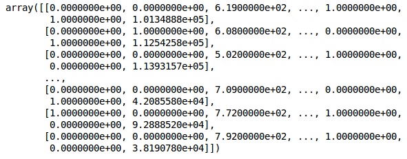
We make the analysis simpler by encoding string variables. We are using the ScikitLearn function ‘LabelEncoder’ to automatically encode the different labels in the columns with values between 0 to n_classes-1.

from sklearn.preprocessing import LabelEncoder, OneHotEncoder
labelencoder_X_1 = LabelEncoder() 
X[:,1] = labelencoder_X_1.fit_transform(X[:,1]) 
labelencoder_X_2 = LabelEncoder() 
X[:, 2] = labelencoder_X_2.fit_transform(X[:, 2])
X

Output

In the above output,country names are replaced by 0, 1 and 2; while male and female are replaced by 0 and 1.

Step 5

Labelling Encoded Data

We use the same ScikitLearn library and another function called the OneHotEncoder to just pass the column number creating a dummy variable.

onehotencoder = OneHotEncoder(categorical features = [1])
X = onehotencoder.fit_transform(X).toarray()
X = X[:, 1:]
X

Now, the first 2 columns represent the country and the 4th column represents the gender.

Output

We always divide our data into training and testing part; we train our model on training data and then we check the accuracy of a model on testing data which helps in evaluating the efficiency of model.

Step 6

We are using ScikitLearn’s train_test_split function to split our data into training set and test set. We keep the train- to- test split ratio as 80:20.

#Splitting the dataset into the Training set and the Test Set
from sklearn.model_selection import train_test_split
X_train, X_test, y_train, y_test = train_test_split(X, y, test_size = 0.2)

Some variables have values in thousands while some have values in tens or ones. We scale the data so that they are more representative.

Step 7

In this code, we are fitting and transforming the training data using the StandardScaler function. We standardize our scaling so that we use the same fitted method to transform/scale test data.

# Feature Scaling

fromsklearn.preprocessing import StandardScaler 
sc = StandardScaler() 
X_train = sc.fit_transform(X_train) 
X_test = sc.transform(X_test)

Output

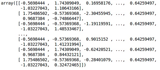
The data is now scaled properly. Finally, we are done with our data pre-processing. Now,we will start with our model.

Step 8

We import the required Modules here. We need the Sequential module for initializing the neural network and the dense module to add the hidden layers.

# Importing the Keras libraries and packages 
import keras 
from keras.models import Sequential 
from keras.layers import Dense

Step 9

We will name the model as Classifier as our aim is to classify customer churn. Then we use the Sequential module for initialization.

#Initializing Neural Network 
classifier = Sequential()

Step 10

We add the hidden layers one by one using the dense function. In the code below, we will see many arguments.

Our first parameter is output_dim. It is the number of nodes we add to this layer. init is the initialization of the Stochastic Gradient Decent. In a Neural Network we assign weights to each node. At initialization, weights should be near to zero and we randomly initialize weights using the uniform function. The input_dim parameter is needed only for first layer, as the model does not know the number of our input variables. Here the total number of input variables is 11. In the second layer, the model automatically knows the number of input variables from the first hidden layer.

Execute the following line of code to addthe input layer and the first hidden layer −

classifier.add(Dense(units = 6, kernel_initializer = 'uniform', 
activation = 'relu', input_dim = 11))

Execute the following line of code to add the second hidden layer −

classifier.add(Dense(units = 6, kernel_initializer = 'uniform', 
activation = 'relu'))

Execute the following line of code to add the output layer −

classifier.add(Dense(units = 1, kernel_initializer = 'uniform', 
activation = 'sigmoid'))

Step 11

Compiling the ANN

We have added multiple layers to our classifier until now. We will now compile them using the compile method. Arguments added in final compilation control complete the neural network.So,we need to be careful in this step.

Here is a brief explanation of the arguments.

First argument is Optimizer.This is an algorithm used to find the optimal set of weights. This algorithm is called the Stochastic Gradient Descent (SGD). Here we are using one among several types, called the ‘Adam optimizer’. The SGD depends on loss, so our second parameter is loss. If our dependent variable is binary, we use logarithmic loss function called ‘binary_crossentropy’, and if our dependent variable has more than two categories in output, then we use ‘categorical_crossentropy’. We want to improve performance of our neural network based on accuracy, so we add metrics as accuracy.

# Compiling Neural Network 
classifier.compile(optimizer = 'adam', loss = 'binary_crossentropy', metrics = ['accuracy'])

Step 12

A number of codes need to be executed in this step.

Fitting the ANN to the Training Set

We now train our model on the training data. We use the fit method to fit our model. We also optimize the weights to improve model efficiency. For this, we have to update the weights. Batch size is the number of observations after which we update the weights. Epoch is the total number of iterations. The values of batch size and epoch are chosen by the trial and error method.

classifier.fit(X_train, y_train, batch_size = 10, epochs = 50)

Making predictions and evaluating the model

# Predicting the Test set results
y_pred = classifier.predict(X_test)
y_pred = (y_pred > 0.5)

Predicting a single new observation

# Predicting a single new observation
"""Our goal is to predict if the customer with the following data will leave the bank:
Geography: Spain
Credit Score: 500
Gender: Female
Age: 40
Tenure: 3
Balance: 50000
Number of Products: 2
Has Credit Card: Yes
Is Active Member: Yes

Step 13

Predicting the test set result

The prediction result will give you probability of the customer leaving the company. We will convert that probability into binary 0 and 1.

# Predicting the Test set results 
y_pred = classifier.predict(X_test) 
y_pred = (y_pred > 0.5)

new_prediction = classifier.predict(sc.transform
(np.array([[0.0, 0, 500, 1, 40, 3, 50000, 2, 1, 1, 40000]])))
new_prediction = (new_prediction > 0.5)

Step 14

This is the last step where we evaluate our model performance. We already have original results and thus we can build confusion matrix to check the accuracy of our model.

Making the Confusion Matrix

from sklearn.metrics import confusion_matrix
cm = confusion_matrix(y_test, y_pred)
print (cm)

Output

loss: 0.3384 acc: 0.8605
[ [1541 54]
[230 175] ]

From the confusion matrix, the Accuracy of our model can be calculated as −

Accuracy = 1541+175/2000=0.858

We achieved 85.8% accuracy, which is good.

The Forward Propagation Algorithm

In this section, we will learn how to write code to do forward propagation (prediction) for a simple neural network −

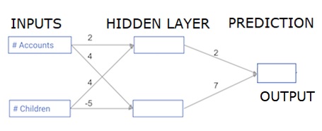
Each data point is a customer. The first input is how many accounts they have, and the second input is how many children they have. The model will predict how many transactions the user makes in the next year.

The input data is pre-loaded as input data, and the weights are in a dictionary called weights. The array of weights for the first node in the hidden layer are in weights [‘node_0’], and for the second node in the hidden layer are in weights[‘node_1’] respectively.

The weights feeding into the output node are available in weights.

The Rectified Linear Activation Function

An "activation function" is a function that works at each node. It transforms the node's input into some output.

The rectified linear activation function (called ReLU) is widely used in very high-performance networks. This function takes a single number as an input, returning 0 if the input is negative, and input as the output if the input is positive.

Here are some examples −

• relu(4) = 4
• relu(-2) = 0

We fill in the definition of the relu() function−

• We use the max() function to calculate the value for the output of relu().
• We apply the relu() function to node_0_input to calculate node_0_output.
• We apply the relu() function to node_1_input to calculate node_1_output.

import numpy as np
input_data = np.array([-1, 2])
weights = {
   'node_0': np.array([3, 3]),
   'node_1': np.array([1, 5]),
   'output': np.array([2, -1])
}
node_0_input = (input_data * weights['node_0']).sum()
node_0_output = np.tanh(node_0_input)
node_1_input = (input_data * weights['node_1']).sum()
node_1_output = np.tanh(node_1_input)
hidden_layer_output = np.array(node_0_output, node_1_output)
output =(hidden_layer_output * weights['output']).sum()
print(output)

def relu(input):
   '''Define your relu activation function here'''
   # Calculate the value for the output of the relu function: output
   output = max(input,0)
      # Return the value just calculated
   return(output)
# Calculate node 0 value: node_0_output
node_0_input = (input_data * weights['node_0']).sum()
node_0_output = relu(node_0_input)

# Calculate node 1 value: node_1_output
node_1_input = (input_data * weights['node_1']).sum()
node_1_output = relu(node_1_input)

# Put node values into array: hidden_layer_outputs
hidden_layer_outputs = np.array([node_0_output, node_1_output])

# Calculate model output (do not apply relu)
odel_output = (hidden_layer_outputs * weights['output']).sum()
print(model_output)# Print model output

Output

0.9950547536867305
-3

Applying the network to many Observations/rows of data

In this section, we will learn how to define a function called predict_with_network(). This function will generate predictions for multiple data observations, taken from network above taken as input_data. The weights given in above network are being used. The relu() function definition is also being used.

Let us define a function called predict_with_network() that accepts two arguments - input_data_row and weights - and returns a prediction from the network as the output.

We calculate the input and output values for each node, storing them as: node_0_input, node_0_output, node_1_input, and node_1_output.

To calculate the input value of a node, we multiply the relevant arrays together and compute their sum.

To calculate the output value of a node, we apply the relu()function to the input value of the node. We use a ‘for loop’ to iterate over input_data −

We also use our predict_with_network() to generate predictions for each row of the input_data - input_data_row. We also append each prediction to results.

# Define predict_with_network()
def predict_with_network(input_data_row, weights):
   # Calculate node 0 value
   node_0_input = (input_data_row * weights['node_0']).sum()
   node_0_output = relu(node_0_input)
   
   # Calculate node 1 value
   node_1_input = (input_data_row * weights['node_1']).sum()
   node_1_output = relu(node_1_input)
   
   # Put node values into array: hidden_layer_outputs
   hidden_layer_outputs = np.array([node_0_output, node_1_output])
   
   # Calculate model output
   input_to_final_layer = (hidden_layer_outputs*weights['output']).sum()
   model_output = relu(input_to_final_layer)
# Return model output
   return(model_output)

# Create empty list to store prediction results
results = []
for input_data_row in input_data:
   # Append prediction to results
   results.append(predict_with_network(input_data_row, weights))
print(results)# Print results

Output

[0, 12]

Here we have used the relu function where relu(26) = 26 and relu(-13)=0 and so on.

Deep multi-layer neural networks

Here we are writing code to do forward propagation for a neural network with two hidden layers. Each hidden layer has two nodes. The input data has been preloaded as input_data. The nodes in the first hidden layer are called node_0_0 and node_0_1.

Their weights are pre-loaded as weights['node_0_0'] and weights['node_0_1'] respectively.

The nodes in the second hidden layer are called node_1_0 and node_1_1. Their weights are pre-loaded as weights['node_1_0'] and weights['node_1_1'] respectively.

We then create a model output from the hidden nodes using weights pre-loaded as weights['output'].

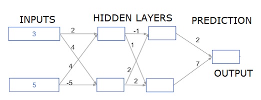
We calculate node_0_0_input using its weights weights['node_0_0'] and the given input_data. Then apply the relu() function to get node_0_0_output.

We do the same as above for node_0_1_input to get node_0_1_output.

We calculate node_1_0_input using its weights weights['node_1_0'] and the outputs from the first hidden layer - hidden_0_outputs. We then apply the relu() function to get node_1_0_output.

We do the same as above for node_1_1_input to get node_1_1_output.

We calculate model_output using weights['output'] and the outputs from the second hidden layer hidden_1_outputs array. We do not apply the relu()function to this output.

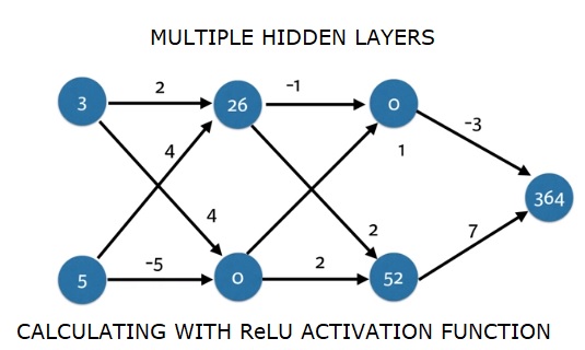
import numpy as np
input_data = np.array([3, 5])
weights = {
   'node_0_0': np.array([2, 4]),
   'node_0_1': np.array([4, -5]),
   'node_1_0': np.array([-1, 1]),
   'node_1_1': np.array([2, 2]),
   'output': np.array([2, 7])
}
def predict_with_network(input_data):
   # Calculate node 0 in the first hidden layer
   node_0_0_input = (input_data * weights['node_0_0']).sum()
   node_0_0_output = relu(node_0_0_input)
   
   # Calculate node 1 in the first hidden layer
   node_0_1_input = (input_data*weights['node_0_1']).sum()
   node_0_1_output = relu(node_0_1_input)
   
   # Put node values into array: hidden_0_outputs
   hidden_0_outputs = np.array([node_0_0_output, node_0_1_output])
   
   # Calculate node 0 in the second hidden layer
   node_1_0_input = (hidden_0_outputs*weights['node_1_0']).sum()
   node_1_0_output = relu(node_1_0_input)
   
   # Calculate node 1 in the second hidden layer
   node_1_1_input = (hidden_0_outputs*weights['node_1_1']).sum()
   node_1_1_output = relu(node_1_1_input)
   
   # Put node values into array: hidden_1_outputs
   hidden_1_outputs = np.array([node_1_0_output, node_1_1_output])
   
   # Calculate model output: model_output
   model_output = (hidden_1_outputs*weights['output']).sum()
      # Return model_output
   return(model_output)
output = predict_with_network(input_data)
print(output)

Output

364