Deep Neural Networks

A deep neural network (DNN) is an ANN with multiple hidden layers between the input and output layers. Similar to shallow ANNs, DNNs can model complex non-linear relationships.

The main purpose of a neural network is to receive a set of inputs, perform progressively complex calculations on them, and give output to solve real world problems like classification. We restrict ourselves to feed forward neural networks.

We have an input, an output, and a flow of sequential data in a deep network.

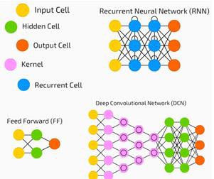
Neural networks are widely used in supervised learning and reinforcement learning problems. These networks are based on a set of layers connected to each other.

In deep learning, the number of hidden layers, mostly non-linear, can be large; say about 1000 layers.

DL models produce much better results than normal ML networks.

We mostly use the gradient descent method for optimizing the network and minimising the loss function.

We can use the Imagenet, a repository of millions of digital images to classify a dataset into categories like cats and dogs. DL nets are increasingly used for dynamic images apart from static ones and for time series and text analysis.

Training the data sets forms an important part of Deep Learning models. In addition, Backpropagation is the main algorithm in training DL models.

DL deals with training large neural networks with complex input output transformations.

One example of DL is the mapping of a photo to the name of the person(s) in photo as they do on social networks and describing a picture with a phrase is another recent application of DL.

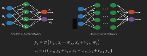
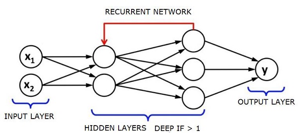
Neural networks are functions that have inputs like x1,x2,x3…that are transformed to outputs like z1,z2,z3 and so on in two (shallow networks) or several intermediate operations also called layers (deep networks).

The weights and biases change from layer to layer. ‘w’ and ‘v’ are the weights or synapses of layers of the neural networks.

The best use case of deep learning is the supervised learning problem.Here,we have large set of data inputs with a desired set of outputs.

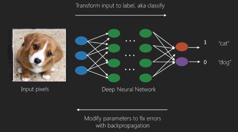
Here we apply back propagation algorithm to get correct output prediction.

The most basic data set of deep learning is the MNIST, a dataset of handwritten digits.

We can train deep a Convolutional Neural Network with Keras to classify images of handwritten digits from this dataset.

The firing or activation of a neural net classifier produces a score. For example,to classify patients as sick and healthy,we consider parameters such as height, weight and body temperature, blood pressure etc.

A high score means patient is sick and a low score means he is healthy.

Each node in output and hidden layers has its own classifiers. The input layer takes inputs and passes on its scores to the next hidden layer for further activation and this goes on till the output is reached.

This progress from input to output from left to right in the forward direction is called forward propagation.

Credit assignment path (CAP) in a neural network is the series of transformations starting from the input to the output. CAPs elaborate probable causal connections between the input and the output.

CAP depth for a given feed forward neural network or the CAP depth is the number of hidden layers plus one as the output layer is included. For recurrent neural networks, where a signal may propagate through a layer several times, the CAP depth can be potentially limitless.

Deep Nets and Shallow Nets

There is no clear threshold of depth that divides shallow learning from deep learning; but it is mostly agreed that for deep learning which has multiple non-linear layers, CAP must be greater than two.

Basic node in a neural net is a perception mimicking a neuron in a biological neural network. Then we have multi-layered Perception or MLP. Each set of inputs is modified by a set of weights and biases; each edge has a unique weight and each node has a unique bias.

The prediction accuracy of a neural net depends on its weights and biases.

The process of improving the accuracy of neural network is called training. The output from a forward prop net is compared to that value which is known to be correct.

The cost function or the loss function is the difference between the generated output and the actual output.

The point of training is to make the cost of training as small as possible across millions of training examples.To do this, the network tweaks the weights and biases until the prediction matches the correct output.

Once trained well, a neural net has the potential to make an accurate prediction every time.

When the pattern gets complex and you want your computer to recognise them, you have to go for neural networks.In such complex pattern scenarios, neural network outperformsall other competing algorithms.

There are now GPUs that can train them faster than ever before. Deep neural networks are already revolutionizing the field of AI

Computers have proved to be good at performing repetitive calculations and following detailed instructions but have been not so good at recognising complex patterns.

If there is the problem of recognition of simple patterns, a support vector machine (svm) or a logistic regression classifier can do the job well, but as the complexity of patternincreases, there is no way but to go for deep neural networks.

Therefore, for complex patterns like a human face, shallow neural networks fail and have no alternative but to go for deep neural networks with more layers. The deep nets are able to do their job by breaking down the complex patterns into simpler ones. For example, human face; adeep net would use edges to detect parts like lips, nose, eyes, ears and so on and then re-combine these together to form a human face

The accuracy of correct prediction has become so accurate that recently at a Google Pattern Recognition Challenge, a deep net beat a human.

This idea of a web of layered perceptrons has been around for some time; in this area, deep nets mimic the human brain. But one downside to this is that they take long time to train, a hardware constraint

However recent high performance GPUs have been able to train such deep nets under a week; while fast cpus could have taken weeks or perhaps months to do the same.

Choosing a Deep Net

How to choose a deep net? We have to decide if we are building a classifier or if we are trying to find patterns in the data and if we are going to use unsupervised learning. To extract patterns from a set of unlabelled data, we use a Restricted Boltzman machine or an Auto encoder.

Consider the following points while choosing a deep net −

For text processing, sentiment analysis, parsing and name entity recognition, we use a recurrent net or recursive neural tensor network or RNTN;
For any language model that operates at character level, we use the recurrent net.
For image recognition, we use deep belief network DBN or convolutional network.
For object recognition, we use a RNTN or a convolutional network.
For speech recognition, we use recurrent net.

In general, deep belief networks and multilayer perceptrons with rectified linear units or RELU are both good choices for classification.

For time series analysis, it is always recommended to use recurrent net.

Neural nets have been around for more than 50 years; but only now they have risen into prominence. The reason is that they are hard to train; when we try to train them with a method called back propagation, we run into a problem called vanishing or exploding gradients.When that happens, training takes a longer time and accuracy takes a back-seat. When training a data set, we are constantly calculating the cost function, which is the difference between predicted output and the actual output from a set of labelled training data.The cost function is then minimized by adjusting the weights and biases values until the lowest value is obtained. The training process uses a gradient, which is the rate at which the cost will change with respect to change in weight or bias values.

Restricted Boltzman Networks or Autoencoders - RBNs

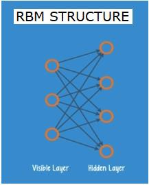
In 2006, a breakthrough was achieved in tackling the issue of vanishing gradients. Geoff Hinton devised a novel strategy that led to the development of Restricted Boltzman Machine - RBM, a shallow two layer net.

The first layer is the visible layer and the second layer is the hidden layer. Each node in the visible layer is connected to every node in the hidden layer. The network is known as restricted as no two layers within the same layer are allowed to share a connection.

Autoencoders are networks that encode input data as vectors. They create a hidden, or compressed, representation of the raw data. The vectors are useful in dimensionality reduction; the vector compresses the raw data into smaller number of essential dimensions. Autoencoders are paired with decoders, which allows the reconstruction of input data based on its hidden representation.

RBM is the mathematical equivalent of a two-way translator. A forward pass takes inputs and translates them into a set of numbers that encodes the inputs. A backward pass meanwhile takes this set of numbers and translates them back into reconstructed inputs. A well-trained net performs back prop with a high degree of accuracy.

In either steps, the weights and the biases have a critical role; they help the RBM in decoding the interrelationships between the inputs and in deciding which inputs are essential in detecting patterns. Through forward and backward passes, the RBM is trained to re-construct the input with different weights and biases until the input and there-construction are as close as possible. An interesting aspect of RBM is that data need not be labelled. This turns out to be very important for real world data sets like photos, videos, voices and sensor data, all of which tend to be unlabelled. Instead of manually labelling data by humans, RBM automatically sorts through data; by properly adjusting the weights and biases, an RBM is able to extract important features and reconstruct the input. RBM is a part of family of feature extractor neural nets, which are designed to recognize inherent patterns in data. These are also called auto-encoders because they have to encode their own structure.

Deep Belief Networks - DBNs

Deep belief networks (DBNs) are formed by combining RBMs and introducing a clever training method. We have a new model that finally solves the problem of vanishing gradient. Geoff Hinton invented the RBMs and also Deep Belief Nets as alternative to back propagation.

A DBN is similar in structure to a MLP (Multi-layer perceptron), but very different when it comes to training. it is the training that enables DBNs to outperform their shallow counterparts

A DBN can be visualized as a stack of RBMs where the hidden layer of one RBM is the visible layer of the RBM above it. The first RBM is trained to reconstruct its input as accurately as possible.

The hidden layer of the first RBM is taken as the visible layer of the second RBM and the second RBM is trained using the outputs from the first RBM. This process is iterated till every layer in the network is trained.

In a DBN, each RBM learns the entire input. A DBN works globally by fine-tuning the entire input in succession as the model slowly improves like a camera lens slowly focussing a picture. A stack of RBMs outperforms a single RBM as a multi-layer perceptron MLP outperforms a single perceptron.

At this stage, the RBMs have detected inherent patterns in the data but without any names or label. To finish training of the DBN, we have to introduce labels to the patterns and fine tune the net with supervised learning.

We need a very small set of labelled samples so that the features and patterns can be associated with a name. This small-labelled set of data is used for training. This set of labelled data can be very small when compared to the original data set.

The weights and biases are altered slightly, resulting in a small change in the net's perception of the patterns and often a small increase in the total accuracy.

The training can also be completed in a reasonable amount of time by using GPUs giving very accurate results as compared to shallow nets and we see a solution to vanishing gradient problem too.

Generative Adversarial Networks - GANs

Generative adversarial networks are deep neural nets comprising two nets, pitted one against the other, thus the “adversarial” name.

GANs were introduced in a paper published by researchers at the University of Montreal in 2014. Facebook’s AI expert Yann LeCun, referring to GANs, called adversarial training “the most interesting idea in the last 10 years in ML.”

GANs’ potential is huge, as the network-scan learn to mimic any distribution of data. GANs can be taught to create parallel worlds strikingly similar to our own in any domain: images, music, speech, prose. They are robot artists in a way, and their output is quite impressive.

In a GAN, one neural network, known as the generator, generates new data instances, while the other, the discriminator, evaluates them for authenticity.

Let us say we are trying to generate hand-written numerals like those found in the MNIST dataset, which is taken from the real world. The work of the discriminator, when shown an instance from the true MNIST dataset, is to recognize them as authentic.

Now consider the following steps of the GAN −

The generator network takes input in the form of random numbers and returns an image.
This generated image is given as input to the discriminator network along with a stream of images taken from the actual dataset.
The discriminator takes in both real and fake images and returns probabilities, a number between 0 and 1, with 1 representing a prediction of authenticity and 0 representing fake.
So you have a double feedback loop −
- The discriminator is in a feedback loop with the ground truth of the images, which we know.
- The generator is in a feedback loop with the discriminator.

Recurrent Neural Networks - RNNs

RNNSare neural networks in which data can flow in any direction. These networks are used for applications such as language modelling or Natural Language Processing (NLP).

The basic concept underlying RNNs is to utilize sequential information. In a normal neural network it is assumed that all inputs and outputs are independent of each other. If we want to predict the next word in a sentence we have to know which words came before it.

RNNs are called recurrent as they repeat the same task for every element of a sequence, with the output being based on the previous computations. RNNs thus can be said to have a “memory” that captures information about what has been previously calculated. In theory, RNNs can use information in very long sequences, but in reality, they can look back only a few steps.

Long short-term memory networks (LSTMs) are most commonly used RNNs.

Together with convolutional Neural Networks, RNNs have been used as part of a model to generate descriptions for unlabelled images. It is quite amazing how well this seems to work.

Convolutional Deep Neural Networks - CNNs

If we increase the number of layers in a neural network to make it deeper, it increases the complexity of the network and allows us to model functions that are more complicated. However, the number of weights and biases will exponentially increase. As a matter of fact, learning such difficult problems can become impossible for normal neural networks. This leads to a solution, the convolutional neural networks.

CNNs are extensively used in computer vision; have been applied also in acoustic modelling for automatic speech recognition.

The idea behind convolutional neural networks is the idea of a “moving filter” which passes through the image. This moving filter, or convolution, applies to a certain neighbourhood of nodes which for example may be pixels, where the filter applied is 0.5 x the node value −

Noted researcher Yann LeCun pioneered convolutional neural networks. Facebook as facial recognition software uses these nets. CNN have been the go to solution for machine vision projects. There are many layers to a convolutional network. In Imagenet challenge, a machine was able to beat a human at object recognition in 2015.

In a nutshell, Convolutional Neural Networks (CNNs) are multi-layer neural networks. The layers are sometimes up to 17 or more and assume the input data to be images.

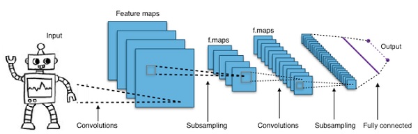
CNNs drastically reduce the number of parameters that need to be tuned. So, CNNs efficiently handle the high dimensionality of raw images.