Part of Speech (PoS) Tagging

Tagging is a kind of classification that may be defined as the automatic assignment of description to the tokens. Here the descriptor is called tag, which may represent one of the part-of-speech, semantic information and so on.

Now, if we talk about Part-of-Speech (PoS) tagging, then it may be defined as the process of assigning one of the parts of speech to the given word. It is generally called POS tagging. In simple words, we can say that POS tagging is a task of labelling each word in a sentence with its appropriate part of speech. We already know that parts of speech include nouns, verb, adverbs, adjectives, pronouns, conjunction and their sub-categories.

Most of the POS tagging falls under Rule Base POS tagging, Stochastic POS tagging and Transformation based tagging.

Rule-based POS Tagging

One of the oldest techniques of tagging is rule-based POS tagging. Rule-based taggers use dictionary or lexicon for getting possible tags for tagging each word. If the word has more than one possible tag, then rule-based taggers use hand-written rules to identify the correct tag. Disambiguation can also be performed in rule-based tagging by analyzing the linguistic features of a word along with its preceding as well as following words. For example, suppose if the preceding word of a word is article then word must be a noun.

As the name suggests, all such kind of information in rule-based POS tagging is coded in the form of rules. These rules may be either −

Context-pattern rules
Or, as Regular expression compiled into finite-state automata, intersected with lexically ambiguous sentence representation.

We can also understand Rule-based POS tagging by its two-stage architecture −

First stage − In the first stage, it uses a dictionary to assign each word a list of potential parts-of-speech.
Second stage − In the second stage, it uses large lists of hand-written disambiguation rules to sort down the list to a single part-of-speech for each word.

Properties of Rule-Based POS Tagging

Rule-based POS taggers possess the following properties −

These taggers are knowledge-driven taggers.
The rules in Rule-based POS tagging are built manually.
The information is coded in the form of rules.
We have some limited number of rules approximately around 1000.
Smoothing and language modeling is defined explicitly in rule-based taggers.

Stochastic POS Tagging

Another technique of tagging is Stochastic POS Tagging. Now, the question that arises here is which model can be stochastic. The model that includes frequency or probability (statistics) can be called stochastic. Any number of different approaches to the problem of part-of-speech tagging can be referred to as stochastic tagger.

The simplest stochastic tagger applies the following approaches for POS tagging −

Word Frequency Approach

In this approach, the stochastic taggers disambiguate the words based on the probability that a word occurs with a particular tag. We can also say that the tag encountered most frequently with the word in the training set is the one assigned to an ambiguous instance of that word. The main issue with this approach is that it may yield inadmissible sequence of tags.

Tag Sequence Probabilities

It is another approach of stochastic tagging, where the tagger calculates the probability of a given sequence of tags occurring. It is also called n-gram approach. It is called so because the best tag for a given word is determined by the probability at which it occurs with the n previous tags.

Properties of Stochastic POST Tagging

Stochastic POS taggers possess the following properties −

This POS tagging is based on the probability of tag occurring.
It requires training corpus
There would be no probability for the words that do not exist in the corpus.
It uses different testing corpus (other than training corpus).
It is the simplest POS tagging because it chooses most frequent tags associated with a word in training corpus.

Transformation-based Tagging

Transformation based tagging is also called Brill tagging. It is an instance of the transformation-based learning (TBL), which is a rule-based algorithm for automatic tagging of POS to the given text. TBL, allows us to have linguistic knowledge in a readable form, transforms one state to another state by using transformation rules.

It draws the inspiration from both the previous explained taggers − rule-based and stochastic. If we see similarity between rule-based and transformation tagger, then like rule-based, it is also based on the rules that specify what tags need to be assigned to what words. On the other hand, if we see similarity between stochastic and transformation tagger then like stochastic, it is machine learning technique in which rules are automatically induced from data.

Working of Transformation Based Learning(TBL)

In order to understand the working and concept of transformation-based taggers, we need to understand the working of transformation-based learning. Consider the following steps to understand the working of TBL −

Start with the solution − The TBL usually starts with some solution to the problem and works in cycles.
Most beneficial transformation chosen − In each cycle, TBL will choose the most beneficial transformation.
Apply to the problem − The transformation chosen in the last step will be applied to the problem.

The algorithm will stop when the selected transformation in step 2 will not add either more value or there are no more transformations to be selected. Such kind of learning is best suited in classification tasks.

Advantages of Transformation-based Learning (TBL)

The advantages of TBL are as follows −

We learn small set of simple rules and these rules are enough for tagging.
Development as well as debugging is very easy in TBL because the learned rules are easy to understand.
Complexity in tagging is reduced because in TBL there is interlacing of machinelearned and human-generated rules.
Transformation-based tagger is much faster than Markov-model tagger.

Disadvantages of Transformation-based Learning (TBL)

The disadvantages of TBL are as follows −

Transformation-based learning (TBL) does not provide tag probabilities.
In TBL, the training time is very long especially on large corpora.

Hidden Markov Model (HMM) POS Tagging

Before digging deep into HMM POS tagging, we must understand the concept of Hidden Markov Model (HMM).

Hidden Markov Model

An HMM model may be defined as the doubly-embedded stochastic model, where the underlying stochastic process is hidden. This hidden stochastic process can only be observed through another set of stochastic processes that produces the sequence of observations.

Example

For example, a sequence of hidden coin tossing experiments is done and we see only the observation sequence consisting of heads and tails. The actual details of the process - how many coins used, the order in which they are selected - are hidden from us. By observing this sequence of heads and tails, we can build several HMMs to explain the sequence. Following is one form of Hidden Markov Model for this problem −

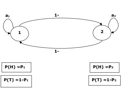
We assumed that there are two states in the HMM and each of the state corresponds to the selection of different biased coin. Following matrix gives the state transition probabilities −

$$A = \begin{bmatrix}a11 & a12 \\a21 & a22 \end{bmatrix}$$

Here,

a_ij = probability of transition from one state to another from i to j.
a₁₁ + a₁₂ = 1 and a₂₁ + a₂₂ =1
P₁ = probability of heads of the first coin i.e. the bias of the first coin.
P₂ = probability of heads of the second coin i.e. the bias of the second coin.

We can also create an HMM model assuming that there are 3 coins or more.

This way, we can characterize HMM by the following elements −

N, the number of states in the model (in the above example N =2, only two states).
M, the number of distinct observations that can appear with each state in the above example M = 2, i.e., H or T).
A, the state transition probability distribution − the matrix A in the above example.
P, the probability distribution of the observable symbols in each state (in our example P1 and P2).
I, the initial state distribution.

Use of HMM for POS Tagging

The POS tagging process is the process of finding the sequence of tags which is most likely to have generated a given word sequence. We can model this POS process by using a Hidden Markov Model (HMM), where tags are the hidden states that produced the observable output, i.e., the words.

Mathematically, in POS tagging, we are always interested in finding a tag sequence (C) which maximizes −

P (C|W)

Where,

C = C₁, C₂, C₃... C_T

W = W₁, W₂, W₃, W_T

On the other side of coin, the fact is that we need a lot of statistical data to reasonably estimate such kind of sequences. However, to simplify the problem, we can apply some mathematical transformations along with some assumptions.

The use of HMM to do a POS tagging is a special case of Bayesian interference. Hence, we will start by restating the problem using Bayes’ rule, which says that the above-mentioned conditional probability is equal to −

(PROB (C₁,..., CT) * PROB (W₁,..., WT | C₁,..., CT)) / PROB (W₁,..., WT)

We can eliminate the denominator in all these cases because we are interested in finding the sequence C which maximizes the above value. This will not affect our answer. Now, our problem reduces to finding the sequence C that maximizes −

PROB (C₁,..., CT) * PROB (W₁,..., WT | C₁,..., CT) (1)

Even after reducing the problem in the above expression, it would require large amount of data. We can make reasonable independence assumptions about the two probabilities in the above expression to overcome the problem.

First Assumption

The probability of a tag depends on the previous one (bigram model) or previous two (trigram model) or previous n tags (n-gram model) which, mathematically, can be explained as follows −

PROB (C₁,..., C_T) = Π_i=1..T PROB (C_i|C_i-n+1…C_i-1) (n-gram model)

PROB (C₁,..., CT) = Π_i=1..T PROB (C_i|C_i-1) (bigram model)

The beginning of a sentence can be accounted for by assuming an initial probability for each tag.

PROB (C₁|C₀) = PROB _initial (C₁)

Second Assumption

The second probability in equation (1) above can be approximated by assuming that a word appears in a category independent of the words in the preceding or succeeding categories which can be explained mathematically as follows −

PROB (W₁,..., W_T | C₁,..., C_T) = Π_i=1..T PROB (W_i|C_i)

Now, on the basis of the above two assumptions, our goal reduces to finding a sequence C which maximizes

Π_i=1...T PROB(C_i|C_i-1) * PROB(W_i|C_i)

Now the question that arises here is has converting the problem to the above form really helped us. The answer is - yes, it has. If we have a large tagged corpus, then the two probabilities in the above formula can be calculated as −

PROB (C_i=VERB|C_i-1=NOUN) = (# of instances where Verb follows Noun) / (# of instances where Noun appears) (2)

PROB (W_i|C_i) = (# of instances where W_i appears in C_i) /(# of instances where C_i appears) (3)