- Modelling & Simulation Tutorial
- Modelling & Simulation - Home
- Introduction
- Concepts & Classification
- Verification & Validation
- Discrete System Simulation
- Continuous Simulation
- Monte Carlo Simulation
- Modelling & Simulation - Database
- Modelling & Simulation Resources
- Quick Guide
- Modelling & Simulation - Resources
- Modelling & Simulation - Discussion
Modelling & Simulation - Quick Guide
Modelling & Simulation - Introduction
Modelling is the process of representing a model which includes its construction and working. This model is similar to a real system, which helps the analyst predict the effect of changes to the system. In other words, modelling is creating a model which represents a system including their properties. It is an act of building a model.
Simulation of a system is the operation of a model in terms of time or space, which helps analyze the performance of an existing or a proposed system. In other words, simulation is the process of using a model to study the performance of a system. It is an act of using a model for simulation.
History of Simulation
The historical perspective of simulation is as enumerated in a chronological order.
1940 − A method named ‘Monte Carlo’ was developed by researchers (John von Neumann, Stanislaw Ulan, Edward Teller, Herman Kahn) and physicists working on a Manhattan project to study neutron scattering.
1960 − The first special-purpose simulation languages were developed, such as SIMSCRIPT by Harry Markowitz at the RAND Corporation.
1970 − During this period, research was initiated on mathematical foundations of simulation.
1980 − During this period, PC-based simulation software, graphical user interfaces and object-oriented programming were developed.
1990 − During this period, web-based simulation, fancy animated graphics, simulation-based optimization, Markov-chain Monte Carlo methods were developed.
Developing Simulation Models
Simulation models consist of the following components: system entities, input variables, performance measures, and functional relationships. Following are the steps to develop a simulation model.
Step 1 − Identify the problem with an existing system or set requirements of a proposed system.
Step 2 − Design the problem while taking care of the existing system factors and limitations.
Step 3 − Collect and start processing the system data, observing its performance and result.
Step 4 − Develop the model using network diagrams and verify it using various verifications techniques.
Step 5 − Validate the model by comparing its performance under various conditions with the real system.
Step 6 − Create a document of the model for future use, which includes objectives, assumptions, input variables and performance in detail.
Step 7 − Select an appropriate experimental design as per requirement.
Step 8 − Induce experimental conditions on the model and observe the result.
Performing Simulation Analysis
Following are the steps to perform simulation analysis.
Step 1 − Prepare a problem statement.
Step 2 − Choose input variables and create entities for the simulation process. There are two types of variables - decision variables and uncontrollable variables. Decision variables are controlled by the programmer, whereas uncontrollable variables are the random variables.
Step 3 − Create constraints on the decision variables by assigning it to the simulation process.
Step 4 − Determine the output variables.
Step 5 − Collect data from the real-life system to input into the simulation.
Step 6 − Develop a flowchart showing the progress of the simulation process.
Step 7 − Choose an appropriate simulation software to run the model.
Step 8 − Verify the simulation model by comparing its result with the real-time system.
Step 9 − Perform an experiment on the model by changing the variable values to find the best solution.
Step 10 − Finally, apply these results into the real-time system.
Modelling & Simulation ─ Advantages
Following are the advantages of using Modelling and Simulation −
Easy to understand − Allows to understand how the system really operates without working on real-time systems.
Easy to test − Allows to make changes into the system and their effect on the output without working on real-time systems.
Easy to upgrade − Allows to determine the system requirements by applying different configurations.
Easy to identifying constraints − Allows to perform bottleneck analysis that causes delay in the work process, information, etc.
Easy to diagnose problems − Certain systems are so complex that it is not easy to understand their interaction at a time. However, Modelling & Simulation allows to understand all the interactions and analyze their effect. Additionally, new policies, operations, and procedures can be explored without affecting the real system.
Modelling & Simulation ─ Disadvantages
Following are the disadvantages of using Modelling and Simulation −
Designing a model is an art which requires domain knowledge, training and experience.
Operations are performed on the system using random number, hence difficult to predict the result.
Simulation requires manpower and it is a time-consuming process.
Simulation results are difficult to translate. It requires experts to understand.
Simulation process is expensive.
Modelling & Simulation ─ Application Areas
Modelling & Simulation can be applied to the following areas − Military applications, training & support, designing semiconductors, telecommunications, civil engineering designs & presentations, and E-business models.
Additionally, it is used to study the internal structure of a complex system such as the biological system. It is used while optimizing the system design such as routing algorithm, assembly line, etc. It is used to test new designs and policies. It is used to verify analytic solutions.
Concepts & Classification
In this chapter, we will discuss various concepts and classification of Modelling.
Models & Events
Following are the basic concepts of Modelling & Simulation.
Object is an entity which exists in the real world to study the behavior of a model.
Base Model is a hypothetical explanation of object properties and its behavior, which is valid across the model.
System is the articulate object under definite conditions, which exists in the real world.
Experimental Frame is used to study a system in the real world, such as experimental conditions, aspects, objectives, etc. Basic Experimental Frame consists of two sets of variables − the Frame Input Variables & the Frame Output Variables, which matches the system or model terminals. The Frame input variable is responsible for matching the inputs applied to the system or a model. The Frame output variable is responsible for matching the output values to the system or a model.
Lumped Model is an exact explanation of a system which follows the specified conditions of a given Experimental Frame.
Verification is the process of comparing two or more items to ensure their accuracy. In Modelling & Simulation, verification can be done by comparing the consistency of a simulation program and the lumped model to ensure their performance. There are various ways to perform validation process, which we will cover in a separate chapter.
Validation is the process of comparing two results. In Modelling & Simulation, validation is performed by comparing experiment measurements with the simulation results within the context of an Experimental Frame. The model is invalid, if the results mismatch. There are various ways to perform validation process, which we will cover in separate chapter.
System State Variables
The system state variables are a set of data, required to define the internal process within the system at a given point of time.
In a discrete-event model, the system state variables remain constant over intervals of time and the values change at defined points called event times.
In continuous-event model, the system state variables are defined by differential equation results whose value changes continuously over time.
Following are some of the system state variables −
Entities & Attributes − An entity represents an object whose value can be static or dynamic, depending upon the process with other entities. Attributes are the local values used by the entity.
Resources − A resource is an entity that provides service to one or more dynamic entities at a time. The dynamic entity can request one or more units of a resource; if accepted then the entity can use the resource and release when completed. If rejected, the entity can join a queue.
Lists − Lists are used to represent the queues used by the entities and resources. There are various possibilities of queues such as LIFO, FIFO, etc. depending upon the process.
Delay − It is an indefinite duration that is caused by some combination of system conditions.
Classification of Models
A system can be classified into the following categories.
Discrete-Event Simulation Model − In this model, the state variable values change only at some discrete points in time where the events occur. Events will only occur at the defined activity time and delays.
Stochastic vs. Deterministic Systems − Stochastic systems are not affected by randomness and their output is not a random variable, whereas deterministic systems are affected by randomness and their output is a random variable.
Static vs. Dynamic Simulation − Static simulation include models which are not affected with time. For example: Monte Carlo Model. Dynamic Simulation include models which are affected with time.
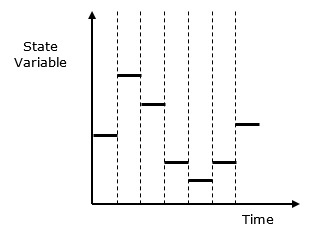
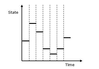
Discrete vs. Continuous Systems − Discrete system is affected by the state variable changes at a discrete point of time. Its behavior is depicted in the following graphical representation.
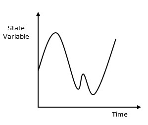
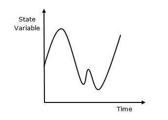
Continuous system is affected by the state variable, which changes continuously as a function with time. Its behavior is depicted in the following graphical representation.
Modelling Process
Modelling process includes the following steps.
Step 1 − Examine the problem. In this stage, we must understand the problem and choose its classification accordingly, such as deterministic or stochastic.
Step 2 − Design a model. In this stage, we have to perform the following simple tasks which help us design a model −
Collect data as per the system behavior and future requirements.
Analyze the system features, its assumptions and necessary actions to be taken to make the model successful.
Determine the variable names, functions, its units, relationships, and their applications used in the model.
Solve the model using a suitable technique and verify the result using verification methods. Next, validate the result.
Prepare a report which includes results, interpretations, conclusion, and suggestions.
Step 3 − Provide recommendations after completing the entire process related to the model. It includes investment, resources, algorithms, techniques, etc.
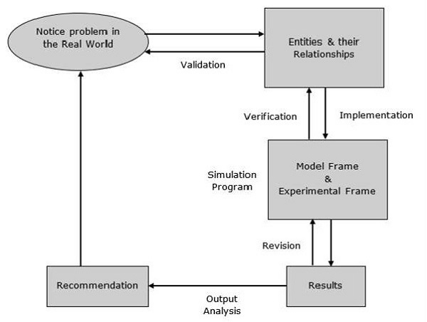
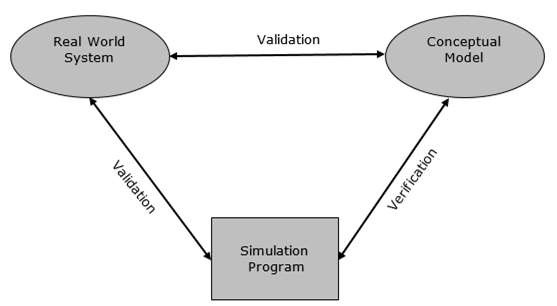
Verification & Validation
One of the real problems that the simulation analyst faces is to validate the model. The simulation model is valid only if the model is an accurate representation of the actual system, else it is invalid.
Validation and verification are the two steps in any simulation project to validate a model.
Validation is the process of comparing two results. In this process, we need to compare the representation of a conceptual model to the real system. If the comparison is true, then it is valid, else invalid.
Verification is the process of comparing two or more results to ensure its accuracy. In this process, we have to compare the model’s implementation and its associated data with the developer's conceptual description and specifications.
Verification & Validation Techniques
There are various techniques used to perform Verification & Validation of Simulation Model. Following are some of the common techniques −
Techniques to Perform Verification of Simulation Model
Following are the ways to perform verification of simulation model −
By using programming skills to write and debug the program in sub-programs.
By using “Structured Walk-through” policy in which more than one person is to read the program.
By tracing the intermediate results and comparing them with observed outcomes.
By checking the simulation model output using various input combinations.
By comparing final simulation result with analytic results.
Techniques to Perform Validation of Simulation Model
Step 1 − Design a model with high validity. This can be achieved using the following steps −
- The model must be discussed with the system experts while designing.
- The model must interact with the client throughout the process.
- The output must supervised by system experts.
Step 2 − Test the model at assumptions data. This can be achieved by applying the assumption data into the model and testing it quantitatively. Sensitive analysis can also be performed to observe the effect of change in the result when significant changes are made in the input data.
Step 3 − Determine the representative output of the Simulation model. This can be achieved using the following steps −
Determine how close is the simulation output with the real system output.
Comparison can be performed using the Turing Test. It presents the data in the system format, which can be explained by experts only.
Statistical method can be used for compare the model output with the real system output.
Model Data Comparison with Real Data
After model development, we have to perform comparison of its output data with real system data. Following are the two approaches to perform this comparison.
Validating the Existing System
In this approach, we use real-world inputs of the model to compare its output with that of the real-world inputs of the real system. This process of validation is straightforward, however, it may present some difficulties when carried out, such as if the output is to be compared to average length, waiting time, idle time, etc. it can be compared using statistical tests and hypothesis testing. Some of the statistical tests are chi-square test, Kolmogorov-Smirnov test, Cramer-von Mises test, and the Moments test.
Validating the First Time Model
Consider we have to describe a proposed system which doesn’t exist at the present nor has existed in the past. Therefore, there is no historical data available to compare its performance with. Hence, we have to use a hypothetical system based on assumptions. Following useful pointers will help in making it efficient.
Subsystem Validity − A model itself may not have any existing system to compare it with, but it may consist of a known subsystem. Each of that validity can be tested separately.
Internal Validity − A model with high degree of internal variance will be rejected as a stochastic system with high variance due to its internal processes will hide the changes in the output due to input changes.
Sensitivity Analysis − It provides the information about the sensitive parameter in the system to which we need to pay higher attention.
Face Validity − When the model performs on opposite logics, then it should be rejected even if it behaves like the real system.
Discrete System Simulation
In discrete systems, the changes in the system state are discontinuous and each change in the state of the system is called an event. The model used in a discrete system simulation has a set of numbers to represent the state of the system, called as a state descriptor. In this chapter, we will also learn about queuing simulation, which is a very important aspect in discrete event simulation along with simulation of time-sharing system.
Following is the graphical representation of the behavior of a discrete system simulation.
Discrete Event Simulation ─ Key Features
Discrete event simulation is generally carried out by a software designed in high level programming languages such as Pascal, C++, or any specialized simulation language. Following are the five key features −
Entities − These are the representation of real elements like the parts of machines.
Relationships − It means to link entities together.
Simulation Executive − It is responsible for controlling the advance time and executing discrete events.
Random Number Generator − It helps to simulate different data coming into the simulation model.
Results & Statistics − It validates the model and provides its performance measures.
Time Graph Representation
Every system depends on a time parameter. In a graphical representation it is referred to as clock time or time counter and initially it is set to zero. Time is updated based on the following two factors −
Time Slicing − It is the time defined by a model for each event until the absence of any event.
Next Event − It is the event defined by the model for the next event to be executed instead of a time interval. It is more efficient than Time Slicing.
Simulation of a Queuing System
A queue is the combination of all entities in the system being served and those waiting for their turn.
Parameters
Following is the list of parameters used in the Queuing System.
| Symbol | Description |
|---|---|
| λ | Denotes the arrival rate which is the number of arrivals per second |
| Ts | Denotes the mean service time for each arrival excluding the waiting time in the queue |
| σTs | Denotes the standard deviation of service time |
| ρ | Denotes the server time utilization, both when it was idle and busy |
| u | Denotes traffic intensity |
| r | Denotes the mean of items in the system |
| R | Denotes the total number of items in the system |
| Tr | Denotes the mean time of an item in the system |
| TR | Denotes the total time of an item in the system |
| σr | Denotes the standard deviation of r |
| σTr | Denotes the standard deviation of Tr |
| w | Denotes the mean number of items waiting in the queue |
| σw | Denotes the standard deviation of w |
| Tw | Denotes the mean waiting time of all items |
| Td | Denotes the mean waiting time of the items waiting in the queue |
| N | Denotes the number of servers in a system |
| mx(y) | Denotes the yth percentile which means the value of y below which x occurs y percent of the time |
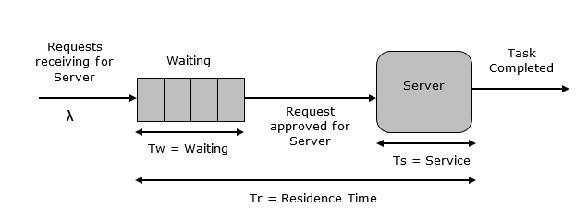
Single Server Queue
This is the simplest queuing system as represented in the following figure. The central element of the system is a server, which provides service to the connected devices or items. Items request to the system to be served, if the server is idle. Then, it is served immediately, else it joins a waiting queue. After the task is completed by the server, the item departs.
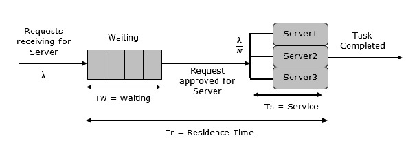
Multi Server Queue
As the name suggests, the system consists of multiple servers and a common queue for all items. When any item requests for the server, it is allocated if at-least one server is available. Else the queue begins to start until the server is free. In this system, we assume that all servers are identical, i.e. there is no difference which server is chosen for which item.
There is an exception of utilization. Let N be the identical servers, then ρ is the utilization of each server. Consider Nρ to be the utilization of the entire system; then the maximum utilization is N*100%, and the maximum input rate is −
$λmax = \frac{\text{N}}{\text{T}s}$
Queuing Relationships
The following table shows some basic queuing relationships.
| General Terms | Single Server | Multi server |
|---|---|---|
| r = λTr Little's formula | ρ = λTs | ρ = λTs/N |
| w = λTw Little's formula | r = w + ρ | u = λTs = ρN |
| Tr = Tw + Ts | r = w + Nρ |
Simulation of Time-Sharing System
Time-sharing system is designed in such a manner that each user uses a small portion of time shared on a system, which results in multiple users sharing the system simultaneously. The switching of each user is so rapid that each user feels like using their own system. It is based on the concept of CPU scheduling and multi-programming where multiple resources can be utilized effectively by executing multiple jobs simultaneously on a system.
Example − SimOS Simulation System.
It is designed by Stanford University to study the complex computer hardware designs, to analyze application performance, and to study the operating systems. SimOS contains software simulation of all the hardware components of the modern computer systems, i.e. processors, Memory Management Units (MMU), caches, etc.
Modelling & Simulation - Continuous
A continuous system is one in which important activities of the system completes smoothly without any delay, i.e. no queue of events, no sorting of time simulation, etc. When a continuous system is modeled mathematically, its variables representing the attributes are controlled by continuous functions.
What is Continuous Simulation?
Continuous simulation is a type of simulation in which state variables change continuously with respect to time. Following is the graphical representation of its behavior.
Why Use Continuous Simulation?
We have to use continuous simulation as it depends on differential equation of various parameters associated with the system and their estimated results known to us.
Application Areas
Continuous simulation is used in the following sectors. In civil engineering for the construction of dam embankment and tunnel constructions. In military applications for simulation of missile trajectory, simulation of fighter aircraft training, and designing & testing of intelligent controller for underwater vehicles.
In logistics for designing of toll plaza, passenger flow analysis at the airport terminal, and proactive flight schedule evaluation. In business development for product development planning, staff management planning, and market study analysis.
Monte Carlo Simulation
Monte Carlo simulation is a computerized mathematical technique to generate random sample data based on some known distribution for numerical experiments. This method is applied to risk quantitative analysis and decision making problems. This method is used by the professionals of various profiles such as finance, project management, energy, manufacturing, engineering, research & development, insurance, oil & gas, transportation, etc.
This method was first used by scientists working on the atom bomb in 1940. This method can be used in those situations where we need to make an estimate and uncertain decisions such as weather forecast predictions.
Monte Carlo Simulation ─ Important Characteristics
Following are the three important characteristics of Monte-Carlo method −
- Its output must generate random samples.
- Its input distribution must be known.
- Its result must be known while performing an experiment.
Monte Carlo Simulation ─ Advantages
- Easy to implement.
- Provides statistical sampling for numerical experiments using the computer.
- Provides approximate solution to mathematical problems.
- Can be used for both stochastic and deterministic problems.
Monte Carlo Simulation ─ Disadvantages
Time consuming as there is a need to generate large number of sampling to get the desired output.
The results of this method are only the approximation of true values, not the exact.
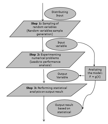
Monte Carlo Simulation Method ─ Flow Diagram
The following illustration shows a generalized flowchart of Monte Carlo simulation.
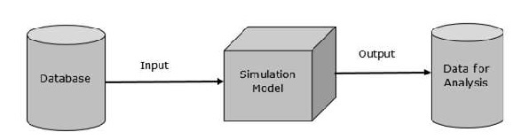
Modelling & Simulation - Database
The objective of the database in Modelling & Simulation is to provide data representation and its relationship for analysis and testing purposes. The first data model was introduced in 1980 by Edgar Codd. Following were the salient features of the model.
Database is the collection of different data objects that defines the information and their relationships.
Rules are for defining the constraints on data in the objects.
Operations can be applied to objects for retrieving information.
Initially, Data Modelling was based on the concept of entities & relationships in which the entities are types of information of data, and relationships represent the associations between the entities.
The latest concept for data modeling is the object-oriented design in which entities are represented as classes, which are used as templates in computer programming. A class having its name, attributes, constraints, and relationships with objects of other classes.
Its basic representation looks like −
Data Representation
Data Representation for Events
A simulation event has its attributes such as the event name and its associated time information. It represents the execution of a provided simulation using a set of input data associated with the input file parameter and provides its result as a set of output data, stored in multiple files associated with data files.
Data Representation for Input Files
Every simulation process requires a different set of input data and its associated parameter values, which are represented in the input data file. The input file is associated with the software which processes the simulation. The data model represents the referenced files by an association with a data file.
Data Representation for Output Files
When the simulation process is completed, it produces various output files and each output file is represented as a data file. Each file has its name, description and a universal factor. A data file is classified into two files. The first file contains the numerical values and the second file contains the descriptive information for the contents of the numerical file.
Neural Networks in Modelling & Simulation
Neural network is the branch of artificial intelligence. Neural network is a network of many processors named as units, each unit having its small local memory. Each unit is connected by unidirectional communication channels named as connections, which carry the numeric data. Each unit works only on their local data and on the inputs they receive from the connections.
History
The historical perspective of simulation is as enumerated in a chronological order.
The first neural model was developed in 1940 by McCulloch & Pitts.
In 1949, Donald Hebb wrote a book “The Organization of Behavior”, which pointed to the concept of neurons.
In 1950, with the computers being advanced, it became possible to make a model on these theories. It was done by IBM research laboratories. However, the effort failed and later attempts were successful.
In 1959, Bernard Widrow and Marcian Hoff, developed models called ADALINE and MADALINE. These models have Multiple ADAptive LINear Elements. MADALINE was the first neural network to be applied to a real-world problem.
In 1962, the perceptron model was developed by Rosenblatt, having the ability to solve simple pattern classification problems.
In 1969, Minsky & Papert provided mathematical proof of the limitations of the perceptron model in computation. It was said that the perceptron model cannot solve X-OR problem. Such drawbacks led to the temporary decline of the neural networks.
In 1982, John Hopfield of Caltech presented his ideas on paper to the National Academy of Sciences to create machines using bidirectional lines. Previously, unidirectional lines were used.
When traditional artificial intelligence techniques involving symbolic methods failed, then arises the need to use neural networks. Neural networks have its massive parallelism techniques, which provide the computing power needed to solve such problems.
Application Areas
Neural network can be used in speech synthesis machines, for pattern recognition, to detect diagnostic problems, in robotic control boards and medical equipments.
Fuzzy Set in Modelling & Simulation
As discussed earlier, each process of continuous simulation depends on differential equations and their parameters such as a, b, c, d > 0. Generally, point estimates are calculated and used in the model. However, sometimes these estimates are uncertain so we need fuzzy numbers in differential equations, which provide the estimates of the unknown parameters.
What is a Fuzzy Set?
In a classical set, an element is either a member of the set or not. Fuzzy sets are defined in terms of classical sets X as −
A = {(x,μA(x))| x ∈ X}
Case 1 − The function μA(x) has the following properties −
∀x ∈ X μA(x) ≥ 0
sup x ∈ X {μA(x)} = 1
Case 2 − Let fuzzy set B be defined as A = {(3, 0.3), (4, 0.7), (5, 1), (6, 0.4)}, then its standard fuzzy notation is written as A = {0.3/3, 0.7/4, 1/5, 0.4/6}
Any value with a membership grade of zero doesn’t appear in the expression of the set.
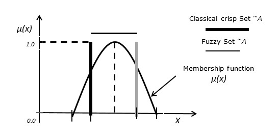
Case 3 − Relationship between fuzzy set and classical crisp set.
The following figure depicts the relationship between a fuzzy set and a classical crisp set.