Discrete System Simulation

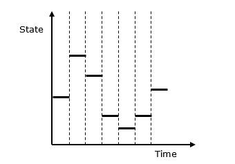
In discrete systems, the changes in the system state are discontinuous and each change in the state of the system is called an event. The model used in a discrete system simulation has a set of numbers to represent the state of the system, called as a state descriptor. In this chapter, we will also learn about queuing simulation, which is a very important aspect in discrete event simulation along with simulation of time-sharing system.

Following is the graphical representation of the behavior of a discrete system simulation.

Discrete Event Simulation ─ Key Features

Discrete event simulation is generally carried out by a software designed in high level programming languages such as Pascal, C++, or any specialized simulation language. Following are the five key features −

Entities − These are the representation of real elements like the parts of machines.
Relationships − It means to link entities together.
Simulation Executive − It is responsible for controlling the advance time and executing discrete events.
Random Number Generator − It helps to simulate different data coming into the simulation model.
Results & Statistics − It validates the model and provides its performance measures.

Time Graph Representation

Every system depends on a time parameter. In a graphical representation it is referred to as clock time or time counter and initially it is set to zero. Time is updated based on the following two factors −

Time Slicing − It is the time defined by a model for each event until the absence of any event.
Next Event − It is the event defined by the model for the next event to be executed instead of a time interval. It is more efficient than Time Slicing.

Simulation of a Queuing System

A queue is the combination of all entities in the system being served and those waiting for their turn.

Parameters

Following is the list of parameters used in the Queuing System.

Symbol	Description
λ	Denotes the arrival rate which is the number of arrivals per second
Ts	Denotes the mean service time for each arrival excluding the waiting time in the queue
σTs	Denotes the standard deviation of service time
ρ	Denotes the server time utilization, both when it was idle and busy
u	Denotes traffic intensity
r	Denotes the mean of items in the system
R	Denotes the total number of items in the system
Tr	Denotes the mean time of an item in the system
TR	Denotes the total time of an item in the system
σr	Denotes the standard deviation of r
σTr	Denotes the standard deviation of Tr
w	Denotes the mean number of items waiting in the queue
σw	Denotes the standard deviation of w
Tw	Denotes the mean waiting time of all items
Td	Denotes the mean waiting time of the items waiting in the queue
N	Denotes the number of servers in a system
mx(y)	Denotes the y^th percentile which means the value of y below which x occurs y percent of the time

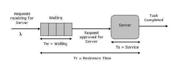
Single Server Queue

This is the simplest queuing system as represented in the following figure. The central element of the system is a server, which provides service to the connected devices or items. Items request to the system to be served, if the server is idle. Then, it is served immediately, else it joins a waiting queue. After the task is completed by the server, the item departs.

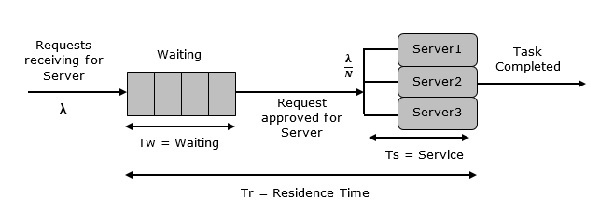
Multi Server Queue

As the name suggests, the system consists of multiple servers and a common queue for all items. When any item requests for the server, it is allocated if at-least one server is available. Else the queue begins to start until the server is free. In this system, we assume that all servers are identical, i.e. there is no difference which server is chosen for which item.

There is an exception of utilization. Let N be the identical servers, then ρ is the utilization of each server. Consider Nρ to be the utilization of the entire system; then the maximum utilization is N*100%, and the maximum input rate is −

$λmax = \frac{\text{N}}{\text{T}s}$

Queuing Relationships

The following table shows some basic queuing relationships.

General Terms	Single Server	Multi server
r = λTr Little's formula	ρ = λTs	ρ = λTs/N
w = λTw Little's formula	r = w + ρ	u = λTs = ρN
Tr = Tw + Ts		r = w + Nρ

Simulation of Time-Sharing System

Time-sharing system is designed in such a manner that each user uses a small portion of time shared on a system, which results in multiple users sharing the system simultaneously. The switching of each user is so rapid that each user feels like using their own system. It is based on the concept of CPU scheduling and multi-programming where multiple resources can be utilized effectively by executing multiple jobs simultaneously on a system.

Example − SimOS Simulation System.

It is designed by Stanford University to study the complex computer hardware designs, to analyze application performance, and to study the operating systems. SimOS contains software simulation of all the hardware components of the modern computer systems, i.e. processors, Memory Management Units (MMU), caches, etc.