- Microsoft Cognitive Toolkit(CNTK) Tutorial
- Home
- Introduction
- Getting Started
- CPU and GPU
- CNTK - Sequence Classification
- CNTK - Logistic Regression Model
- CNTK - Neural Network (NN) Concepts
- CNTK - Creating First Neural Network
- CNTK - Training the Neural Network
- CNTK - In-Memory and Large Datasets
- CNTK - Measuring Performance
- Neural Network Classification
- Neural Network Binary Classification
- CNTK - Neural Network Regression
- CNTK - Classification Model
- CNTK - Regression Model
- CNTK - Out-of-Memory Datasets
- CNTK - Monitoring the Model
- CNTK - Convolutional Neural Network
- CNTK - Recurrent Neural Network
- Microsoft Cognitive Toolkit Resources
- Microsoft Cognitive Toolkit - Quick Guide
- Microsoft Cognitive Toolkit - Resources
- Microsoft Cognitive Toolkit - Discussion
Microsoft Cognitive Toolkit - Quick Guide
Microsoft Cognitive Toolkit (CNTK) - Introduction
In this chapter, we will learn what is CNTK, its features, difference between its version 1.0 and 2.0 and important highlights of version 2.7.
What is Microsoft Cognitive Toolkit (CNTK)?
Microsoft Cognitive Toolkit (CNTK), formerly known as Computational Network Toolkit, is a free, easy-to-use, open-source, commercial-grade toolkit that enables us to train deep learning algorithms to learn like the human brain. It enables us to create some popular deep learning systems like feed-forward neural network time series prediction systems and Convolutional neural network (CNN) image classifiers.
For optimal performance, its framework functions are written in C++. Although we can call its function using C++, but the most commonly used approach for the same is to use a Python program.
CNTK’s Features
Following are some of the features and capabilities offered in the latest version of Microsoft CNTK:
Built-in components
CNTK has highly optimised built-in components that can handle multi-dimensional dense or sparse data from Python, C++ or BrainScript.
We can implement CNN, FNN, RNN, Batch Normalisation and Sequence-to-Sequence with attention.
It provides us the functionality to add new user-defined core-components on the GPU from Python.
It also provides automatic hyperparameter tuning.
We can implement Reinforcement learning, Generative Adversarial Networks (GANs), Supervised as well as Unsupervised learning.
For massive datasets, CNTK has built-in optimised readers.
Usage of resources efficiently
CNTK provides us parallelism with high accuracy on multiple GPUs/machines via 1-bit SGD.
To fit the largest models in GPU memory, it provides memory sharing and other built-in methods.
Express our own networks easily
CNTK has full APIs for defining your own network, learners, readers, training and evaluation from Python, C++, and BrainScript.
Using CNTK, we can easily evaluate models with Python, C++, C# or BrainScript.
It provides both high-level as well as low-level APIs.
Based on our data, it can automatically shape the inference.
It has fully optimised symbolic Recurrent Neural Network (RNN) loops.
Measuring model performance
CNTK provides various components to measure the performance of neural networks you build.
Generates log data from your model and the associated optimiser, which we can use to monitor the training process.
Version 1.0 vs Version 2.0
Following table compares CNTK Version 1.0 and 2.0:
| Version 1.0 | Version 2.0 |
|---|---|
| It was released in 2016. | It is a significant rewrite of the 1.0 Version and was released in June 2017. |
| It used a proprietary scripting language called BrainScript. | Its framework functions can be called using C++, Python. We can easily load our modules in C# or Java. BrainScript is also supported by Version 2.0. |
| It runs on both Windows and Linux systems but not directly on Mac OS. | It also runs on both Windows (Win 8.1, Win 10, Server 2012 R2 and later) and Linux systems but not directly on Mac OS. |
Important Highlights of Version 2.7
Version 2.7 is the last main released version of Microsoft Cognitive Toolkit. It has full support for ONNX 1.4.1. Following are some important highlights of this last released version of CNTK.
Full support for ONNX 1.4.1.
Support for CUDA 10 for both Windows and Linux systems.
It supports advance Recurrent Neural Networks (RNN) loop in ONNX export.
It can export more than 2GB models in ONNX format.
It supports FP16 in BrainScript scripting language’s training action.
Microsoft Cognitive Toolkit (CNTK) - Getting Started
Here, we will understand about the installation of CNTK on Windows and on Linux. Moreover, the chapter explains installing CNTK package, steps to install Anaconda, CNTK files, directory structure and CNTK library organisation.
Prerequisites
In order to install CNTK, we must have Python installed on our computers. You can go to the link https://www.python.org/downloads/ and select the latest version for your OS, i.e. Windows and Linux/Unix. For basic tutorial on Python, you can refer to the link https://www.tutorialspoint.com/python3/index.htm.

CNTK is supported for Windows as well as Linux so we will walk through both of them.
Installing on Windows
In order to run CNTK on Windows, we will be using the Anaconda version of Python. We know that, Anaconda is a redistribution of Python. It includes additional packages like Scipy andScikit-learn which are used by CNTK to perform various useful calculations.
So, first let see the steps to install Anaconda on your machine −
Step 1−First download the setup files from the public website https://www.anaconda.com/distribution/.
Step 2 − Once you downloaded the setup files, start the installation and follow the instructions from the link https://docs.anaconda.com/anaconda/install/.
Step 3 − Once installed, Anaconda will also install some other utilities, which will automatically include all the Anaconda executables in your computer PATH variable. We can manage our Python environment from this prompt, can install packages and run Python scripts.
Installing CNTK package
Once Anaconda installation is done, you can use the most common way to install the CNTK package through the pip executable by using following command −
pip install cntk
There are various other methods to install Cognitive Toolkit on your machine. Microsoft has a neat set of documentation that explains the other installation methods in detail. Please follow the link https://docs.microsoft.com/en-us/cognitive-toolkit/Setup-CNTK-on-your-machine.
Installing on Linux
Installation of CNTK on Linux is a bit different from its installation on Windows. Here, for Linux we are going to use Anaconda to install CNTK, but instead of a graphical installer for Anaconda, we will be using a terminal-based installer on Linux. Although, the installer will work with almost all Linux distributions, we limited the description to Ubuntu.
So, first let see the steps to install Anaconda on your machine −
Steps to install Anaconda
Step 1 − Before installing Anaconda, make sure that the system is fully up to date. To check, first execute the following two commands inside a terminal −
sudo apt update
sudo apt upgrade
Step 2 − Once the computer is updated, get the URL from the public website https://www.anaconda.com/distribution/ for the latest Anaconda installation files.
Step 3 − Once URL is copied, open a terminal window and execute the following command −
wget -0 anaconda-installer.sh url SHAPE \* MERGEFORMAT
     y


	             f


      x

|                     }
Replace the url placeholder with the URL copied from the Anaconda website.
Step 4 − Next, with the help of following command, we can install Anaconda −
sh ./anaconda-installer.sh
The above command will by default install Anaconda3 inside our home directory.
Installing CNTK package
Once Anaconda installation is done, you can use the most common way to install the CNTK package through the pip executable by using following command −
pip install cntk
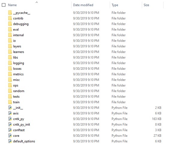
Examining CNTK files & directory structure
Once CNTK is installed as a Python package, we can examine its file and directory structure. It’s at C:\Users\
Verifying CNTK installation
Once CNTK is installed as a Python package, you should verify that CNTK has been installed correctly. From Anaconda command shell, start Python interpreter by entering ipython. Then, import CNTK by entering the following command.
import cntk as c
Once imported, check its version with the help of following command −
print(c.__version__)
The interpreter will respond with installed CNTK version. If it doesn’t respond, there will be a problem with the installation.
The CNTK library organisation
CNTK, a python package technically, is organised into 13 high-level sub-packages and 8 smaller sub-packages. Following table consist of the 10 most frequently used packages:
| Sr.No | Package Name & Description |
|---|---|
| 1 |
cntk.io Contains functions for reading data. For example: next_minibatch() |
| 2 |
cntk.layers Contains high-level functions for creating neural networks. For example: Dense() |
| 3 |
cntk.learners Contains functions for training. For example: sgd() |
| 4 |
cntk.losses Contains functions to measure training error. For example: squared_error() |
| 5 |
cntk.metrics Contains functions to measure model error. For example: classificatoin_error |
| 6 |
cntk.ops Contains low-level functions for creating neural networks. For example: tanh() |
| 7 |
cntk.random Contains functions to generate random numbers. For example: normal() |
| 8 |
cntk.train Contains training functions. For example: train_minibatch() |
| 9 |
cntk.initializer Contains model parameter initializers. For example: normal() and uniform() |
| 10 |
cntk.variables Contains low-level constructs. For example: Parameter() and Variable() |
Microsoft Cognitive Toolkit (CNTK) - CPU and GPU
Microsoft Cognitive Toolkit offers two different build versions namely CPU-only and GPU-only.
CPU only build version
The CPU-only build version of CNTK uses the optimised Intel MKLML, where MKLML is the subset of MKL (Math Kernel Library) and released with Intel MKL-DNN as a terminated version of Intel MKL for MKL-DNN.
GPU only build version
On the other hand, the GPU-only build version of CNTK uses highly optimised NVIDIA libraries such as CUB and cuDNN. It supports distributed training across multiple GPUs and multiple machines. For even faster distributed training in CNTK, the GPU-build version also includes −
MSR-developed 1bit-quantized SGD.
Block-momentum SGD parallel training algorithms.
Enabling GPU with CNTK on Windows
In the previous section, we saw how to install the basic version of CNTK to use with the CPU. Now let’s discuss how we can install CNTK to use with a GPU. But, before getting deep dive into it, first you should have a supported graphics card.
At present, CNTK supports the NVIDIA graphics card with at least CUDA 3.0 support. To make sure, you can check at https://developer.nvidia.com/cuda-gpus whether your GPU supports CUDA.
So, let us see the steps to enable GPU with CNTK on Windows OS −
Step 1 − Depending on the graphics card you are using, first you need to have the latest GeForce or Quadro drivers for your graphics card.
Step 2 − Once you downloaded the drivers, you need to install the CUDA toolkit Version 9.0 for Windows from NVIDIA website https://developer.nvidia.com/cuda-90-download-archive?target_os=Windows&target_arch=x86_64. After installing, run the installer and follow the instructions.
Step 3 − Next, you need to install cuDNN binaries from NVIDIA website https://developer.nvidia.com/rdp/form/cudnn-download-survey. With CUDA 9.0 version, cuDNN 7.4.1 works well. Basically, cuDNN is a layer on the top of CUDA, used by CNTK.
Step 4 − After downloading the cuDNN binaries, you need to extract the zip file into the root folder of your CUDA toolkit installation.
Step 5 − This is the last step which will enable GPU usage inside CNTK. Execute the following command inside the Anaconda prompt on Windows OS −
pip install cntk-gpu
Enabling GPU with CNTK on Linux
Let us see how we can enable GPU with CNTK on Linux OS −
Downloading the CUDA toolkit
First, you need to install the CUDA toolkit from NVIDIA website https://developer.nvidia.com/cuda-90-download-archive?target_os=Linux&target_arch=x86_64&target_distro=Ubuntu&target_version=1604&target_type =runfilelocal.
Running the installer
Now, once you have binaries on the disk, run the installer by opening a terminal and executing the following command and the instruction on screen −
sh cuda_9.0.176_384.81_linux-run
Modify Bash profile script
After installing CUDA toolkit on your Linux machine, you need to modify the BASH profile script. For this, first open the $HOME/ .bashrc file in text editor. Now, at the end of the script, include the following lines −
export PATH=/usr/local/cuda-9.0/bin${PATH:+:${PATH}}
export LD_LIBRARY_PATH=/usr/local/cuda-9.0/lib64\
${LD_LIBRARY_PATH:+:${LD_LIBRARY_PATH}}
Installing
Installing cuDNN libraries
At last we need to install cuDNN binaries. It can be downloaded from NVIDIA website https://developer.nvidia.com/rdp/form/cudnn-download-survey. With CUDA 9.0 version, cuDNN 7.4.1 works well. Basically, cuDNN is a layer on the top of CUDA, used by CNTK.
Once downloaded the version for Linux, extract it to the /usr/local/cuda-9.0 folder by using the following command −
tar xvzf -C /usr/local/cuda-9.0/ cudnn-9.0-linux-x64-v7.4.1.5.tgz
Change the path to the filename as required.
CNTK - Sequence Classification
In this chapter, we will learn in detail about the sequences in CNTK and its classification.
Tensors
The concept on which CNTK works is tensor. Basically, CNTK inputs, outputs as well as parameters are organized as tensors, which is often thought of as a generalised matrix. Every tensor has a rank −
Tensor of rank 0 is a scalar.
Tensor of rank 1 is a vector.
Tensor of rank 2 is amatrix.
Here, these different dimensions are referred as axes.
Static axes and Dynamic axes
As the name implies, the static axes have the same length throughout the network’s life. On the other hand, the length of dynamic axes can vary from instance to instance. In fact, their length is typically not known before each minibatch is presented.
Dynamic axes are like static axes because they also define a meaningful grouping of the numbers contained in the tensor.
Example
To make it clearer, let’s see how a minibatch of short video clips is represented in CNTK. Suppose that the resolution of video clips is all 640 * 480. And, also the clips are shot in color which is typically encoded with three channels. It further means that our minibatch has the following −
3 static axes of length 640, 480 and 3 respectively.
Two dynamic axes; the length of the video and the minibatch axes.
It means that if a minibatch is having 16 videos each of which is 240 frames long, would be represented as 16*240*3*640*480 tensors.
Working with sequences in CNTK
Let us understand sequences in CNTK by first learning about Long-Short Term Memory Network.
Long-Short Term Memory Network (LSTM)

Long-short term memory (LSTMs) networks were introduced by Hochreiter & Schmidhuber. It solved the problem of getting a basic recurrent layer to remember things for a long time. The architecture of LSTM is given above in the diagram. As we can see it has input neurons, memory cells, and output neurons. In order to combat the vanishing gradient problem, Long-short term memory networks use an explicit memory cell (stores the previous values) and the following gates −
Forget gate − As the name implies, it tells the memory cell to forget the previous values. The memory cell stores the values until the gate i.e. ‘forget gate’ tells it to forget them.
Input gate − As name implies, it adds new stuff to the cell.
Output gate − As name implies, output gate decides when to pass along the vectors from the cell to the next hidden state.
It is very easy to work with sequences in CNTK. Let’s see it with the help of following example −
import sys
import os
from cntk import Trainer, Axis
from cntk.io import MinibatchSource, CTFDeserializer, StreamDef, StreamDefs,\
   INFINITELY_REPEAT
from cntk.learners import sgd, learning_parameter_schedule_per_sample
from cntk import input_variable, cross_entropy_with_softmax, \
   classification_error, sequence
from cntk.logging import ProgressPrinter
from cntk.layers import Sequential, Embedding, Recurrence, LSTM, Dense
def create_reader(path, is_training, input_dim, label_dim):
   return MinibatchSource(CTFDeserializer(path, StreamDefs(
      features=StreamDef(field='x', shape=input_dim, is_sparse=True),
      labels=StreamDef(field='y', shape=label_dim, is_sparse=False)
   )), randomize=is_training,
   max_sweeps=INFINITELY_REPEAT if is_training else 1)
def LSTM_sequence_classifier_net(input, num_output_classes, embedding_dim,
LSTM_dim, cell_dim):
   lstm_classifier = Sequential([Embedding(embedding_dim),
      Recurrence(LSTM(LSTM_dim, cell_dim)),
      sequence.last,
      Dense(num_output_classes)])
return lstm_classifier(input)
def train_sequence_classifier():
   input_dim = 2000
   cell_dim = 25
   hidden_dim = 25
   embedding_dim = 50
   num_output_classes = 5
   features = sequence.input_variable(shape=input_dim, is_sparse=True)
   label = input_variable(num_output_classes)
   classifier_output = LSTM_sequence_classifier_net(
   features, num_output_classes, embedding_dim, hidden_dim, cell_dim)
   ce = cross_entropy_with_softmax(classifier_output, label)
   pe =      classification_error(classifier_output, label)
   rel_path = ("../../../Tests/EndToEndTests/Text/" +
      "SequenceClassification/Data/Train.ctf")
   path = os.path.join(os.path.dirname(os.path.abspath(__file__)), rel_path)
   reader = create_reader(path, True, input_dim, num_output_classes)
input_map = {
   features: reader.streams.features,
   label: reader.streams.labels
}
lr_per_sample = learning_parameter_schedule_per_sample(0.0005)
progress_printer = ProgressPrinter(0)
trainer = Trainer(classifier_output, (ce, pe),
sgd(classifier_output.parameters, lr=lr_per_sample),progress_printer)
minibatch_size = 200
for i in range(255):
   mb = reader.next_minibatch(minibatch_size, input_map=input_map)
trainer.train_minibatch(mb)
   evaluation_average = float(trainer.previous_minibatch_evaluation_average)
   loss_average = float(trainer.previous_minibatch_loss_average)
return evaluation_average, loss_average
if __name__ == '__main__':
   error, _ = train_sequence_classifier()
   print(" error: %f" % error)
average  since  average  since  examples
loss     last   metric   last
------------------------------------------------------
1.61    1.61    0.886     0.886     44
1.61     1.6    0.714     0.629    133
 1.6    1.59     0.56     0.448    316
1.57    1.55    0.479      0.41    682
1.53     1.5    0.464     0.449   1379
1.46     1.4    0.453     0.441   2813
1.37    1.28     0.45     0.447   5679
 1.3    1.23    0.448     0.447  11365

error: 0.333333
The detailed explanation of the above program will be covered in next sections, especially when we will be constructing Recurrent Neural networks.
CNTK - Logistic Regression Model
This chapter deals with constructing a logistic regression model in CNTK.
Basics of Logistic Regression model
Logistic Regression, one of the simplest ML techniques, is a technique especially for binary classification. In other words, to create a prediction model in situations where the value of the variable to predict can be one of just two categorical values. One of the simplest examples of Logistic Regression is to predict whether the person is male or female, based on person’s age, voice, hairs and so on.
Example
Let’s understand the concept of Logistic Regression mathematically with the help of another example −
Suppose, we want to predict the credit worthiness of a loan application; 0 means reject, and 1 means approve, based on applicant debt , income and credit rating. We represent debt with X1, income with X2 and credit rating with X3.
In Logistic Regression, we determine a weight value, represented by w, for every feature and a single bias value, represented by b.
Now suppose,
X1 = 3.0
X2 = -2.0
X3 = 1.0
And suppose we determine weight and bias as follows −
W1 = 0.65, W2 = 1.75, W3 = 2.05 and b = 0.33
Now, for predicting the class, we need to apply the following formula −
Z = (X1*W1)+(X2*W2)+(X3+W3)+b
i.e. Z = (3.0)*(0.65) + (-2.0)*(1.75) + (1.0)*(2.05) + 0.33
= 0.83
Next, we need to compute P = 1.0/(1.0 + exp(-Z)). Here, the exp() function is Euler’s number.
P = 1.0/(1.0 + exp(-0.83)
= 0.6963
The P value can be interpreted as the probability that the class is 1. If P < 0.5, the prediction is class = 0 else the prediction (P >= 0.5) is class = 1.
To determine the values of weight and bias, we must obtain a set of training data having the known input predictor values and known correct class labels values. After that, we can use an algorithm, generally Gradient Descent, in order to find the values of weight and bias.
LR model implementation example
For this LR model, we are going to use the following data set −
1.0, 2.0, 0
3.0, 4.0, 0
5.0, 2.0, 0
6.0, 3.0, 0
8.0, 1.0, 0
9.0, 2.0, 0
1.0, 4.0, 1
2.0, 5.0, 1
4.0, 6.0, 1
6.0, 5.0, 1
7.0, 3.0, 1
8.0, 5.0, 1
To start this LR model implementation in CNTK, we need to first import the following packages −
import numpy as np
import cntk as C
The program is structured with main() function as follows −
def main():
print("Using CNTK version = " + str(C.__version__) + "\n")
Now, we need to load the training data into memory as follows −
data_file = ".\\dataLRmodel.txt"
print("Loading data from " + data_file + "\n")
features_mat = np.loadtxt(data_file, dtype=np.float32, delimiter=",", skiprows=0, usecols=[0,1])
labels_mat = np.loadtxt(data_file, dtype=np.float32, delimiter=",", skiprows=0, usecols=[2], ndmin=2)
Now, we will be creating a training program that creates a logistic regression model which is compatible with the training data −
features_dim = 2
labels_dim = 1
X = C.ops.input_variable(features_dim, np.float32)
y = C.input_variable(labels_dim, np.float32)
W = C.parameter(shape=(features_dim, 1)) # trainable cntk.Parameter
b = C.parameter(shape=(labels_dim))
z = C.times(X, W) + b
p = 1.0 / (1.0 + C.exp(-z))
model = p
Now, we need to create Lerner and trainer as follows −
ce_error = C.binary_cross_entropy(model, y) # CE a bit more principled for LR
fixed_lr = 0.010
learner = C.sgd(model.parameters, fixed_lr)
trainer = C.Trainer(model, (ce_error), [learner])
max_iterations = 4000
LR Model training
Once, we have created the LR model, next, it is time to start the training process −
np.random.seed(4)
N = len(features_mat)
for i in range(0, max_iterations):
row = np.random.choice(N,1) # pick a random row from training items
trainer.train_minibatch({ X: features_mat[row], y: labels_mat[row] })
if i % 1000 == 0 and i > 0:
mcee = trainer.previous_minibatch_loss_average
print(str(i) + " Cross-entropy error on curr item = %0.4f " % mcee)
Now, with the help of the following code, we can print the model weights and bias −
np.set_printoptions(precision=4, suppress=True)
print("Model weights: ")
print(W.value)
print("Model bias:")
print(b.value)
print("")
if __name__ == "__main__":
main()
Training a Logistic Regression model - Complete example
import numpy as np
import cntk as C
   def main():
print("Using CNTK version = " + str(C.__version__) + "\n")
data_file = ".\\dataLRmodel.txt" # provide the name and the location of data file
print("Loading data from " + data_file + "\n")
features_mat = np.loadtxt(data_file, dtype=np.float32, delimiter=",", skiprows=0, usecols=[0,1])
labels_mat = np.loadtxt(data_file, dtype=np.float32, delimiter=",", skiprows=0, usecols=[2], ndmin=2)
features_dim = 2
labels_dim = 1
X = C.ops.input_variable(features_dim, np.float32)
y = C.input_variable(labels_dim, np.float32)
W = C.parameter(shape=(features_dim, 1)) # trainable cntk.Parameter
b = C.parameter(shape=(labels_dim))
z = C.times(X, W) + b
p = 1.0 / (1.0 + C.exp(-z))
model = p
ce_error = C.binary_cross_entropy(model, y) # CE a bit more principled for LR
fixed_lr = 0.010
learner = C.sgd(model.parameters, fixed_lr)
trainer = C.Trainer(model, (ce_error), [learner])
max_iterations = 4000
np.random.seed(4)
N = len(features_mat)
for i in range(0, max_iterations):
row = np.random.choice(N,1) # pick a random row from training items
trainer.train_minibatch({ X: features_mat[row], y: labels_mat[row] })
if i % 1000 == 0 and i > 0:
mcee = trainer.previous_minibatch_loss_average
print(str(i) + " Cross-entropy error on curr item = %0.4f " % mcee)
np.set_printoptions(precision=4, suppress=True)
print("Model weights: ")
print(W.value)
print("Model bias:")
print(b.value)
if __name__ == "__main__":
  main()
Output
Using CNTK version = 2.7
1000 cross entropy error on curr item = 0.1941
2000 cross entropy error on curr item = 0.1746
3000 cross entropy error on curr item = 0.0563
Model weights:
[-0.2049]
   [0.9666]]
Model bias:
[-2.2846]
Prediction using trained LR Model
Once the LR model has been trained, we can use it for prediction as follows −
First of all, our evaluation program imports the numpy package and loads the training data into a feature matrix and a class label matrix in the same way as the training program we implement above −
import numpy as np
def main():
data_file = ".\\dataLRmodel.txt" # provide the name and the location of data file
features_mat = np.loadtxt(data_file, dtype=np.float32, delimiter=",",
skiprows=0, usecols=(0,1))
labels_mat = np.loadtxt(data_file, dtype=np.float32, delimiter=",",
skiprows=0, usecols=[2], ndmin=2)
Next, it is time to set the values of the weights and the bias that were determined by our training program −
print("Setting weights and bias values \n")
weights = np.array([0.0925, 1.1722], dtype=np.float32)
bias = np.array([-4.5400], dtype=np.float32)
N = len(features_mat)
features_dim = 2
Next our evaluation program will compute the logistic regression probability by walking through each training items as follows −
print("item pred_prob pred_label act_label result")
for i in range(0, N): # each item
   x = features_mat[i]
   z = 0.0
   for j in range(0, features_dim):
   z += x[j] * weights[j]
   z += bias[0]
   pred_prob = 1.0 / (1.0 + np.exp(-z))
  pred_label = 0 if pred_prob < 0.5 else 1
   act_label = labels_mat[i]
   pred_str = ‘correct’ if np.absolute(pred_label - act_label) < 1.0e-5 \
    else ‘WRONG’
  print("%2d %0.4f %0.0f %0.0f %s" % \ (i, pred_prob, pred_label, act_label, pred_str))
Now let us demonstrate how to do prediction −
x = np.array([9.5, 4.5], dtype=np.float32)
print("\nPredicting class for age, education = ")
print(x)
z = 0.0
for j in range(0, features_dim):
z += x[j] * weights[j]
z += bias[0]
p = 1.0 / (1.0 + np.exp(-z))
print("Predicted p = " + str(p))
if p < 0.5: print("Predicted class = 0")
else: print("Predicted class = 1")
Complete prediction evaluation program
import numpy as np
def main():
data_file = ".\\dataLRmodel.txt" # provide the name and the location of data file
features_mat = np.loadtxt(data_file, dtype=np.float32, delimiter=",",
skiprows=0, usecols=(0,1))
labels_mat = np.loadtxt(data_file, dtype=np.float32, delimiter=",",
skiprows=0, usecols=[2], ndmin=2)
print("Setting weights and bias values \n")
weights = np.array([0.0925, 1.1722], dtype=np.float32)
bias = np.array([-4.5400], dtype=np.float32)
N = len(features_mat)
features_dim = 2
print("item pred_prob pred_label act_label result")
for i in range(0, N): # each item
   x = features_mat[i]
   z = 0.0
   for j in range(0, features_dim):
     z += x[j] * weights[j]
   z += bias[0]
   pred_prob = 1.0 / (1.0 + np.exp(-z))
   pred_label = 0 if pred_prob < 0.5 else 1
   act_label = labels_mat[i]
   pred_str = ‘correct’ if np.absolute(pred_label - act_label) < 1.0e-5 \
     else ‘WRONG’
  print("%2d %0.4f %0.0f %0.0f %s" % \ (i, pred_prob, pred_label, act_label, pred_str))
x = np.array([9.5, 4.5], dtype=np.float32)
print("\nPredicting class for age, education = ")
print(x)
z = 0.0
for j in range(0, features_dim):
   z += x[j] * weights[j]
z += bias[0]
p = 1.0 / (1.0 + np.exp(-z))
print("Predicted p = " + str(p))
if p < 0.5: print("Predicted class = 0")
else: print("Predicted class = 1")
if __name__ == "__main__":
  main()
Output
Setting weights and bias values.
Item  pred_prob  pred_label  act_label  result
0   0.3640         0             0     correct
1   0.7254         1             0      WRONG
2   0.2019         0             0     correct
3   0.3562         0             0     correct
4   0.0493         0             0     correct
5   0.1005         0             0     correct
6   0.7892         1             1     correct
7   0.8564         1             1     correct
8   0.9654         1             1     correct
9   0.7587         1             1     correct
10  0.3040         0             1      WRONG
11  0.7129         1             1     correct
Predicting class for age, education =
[9.5 4.5]
Predicting p = 0.526487952
Predicting class = 1
CNTK - Neural Network (NN) Concepts
This chapter deals with concepts of Neural Network with regards to CNTK.
As we know that, several layers of neurons are used for making a neural network. But, the question arises that in CNTK how we can model the layers of a NN? It can be done with the help of layer functions defined in the layer module.
Layer function
Actually, in CNTK, working with the layers has a distinct functional programming feel to it. Layer function looks like a regular function and it produces a mathematical function with a set of predefined parameters. Let’s see how we can create the most basic layer type, Dense, with the help of layer function.
Example
With the help of following basic steps, we can create the most basic layer type −
Step 1 − First, we need to import the Dense layer function from the layers’ package of CNTK.
from cntk.layers import Dense
Step 2 − Next from the CNTK root package, we need to import the input_variable function.
from cntk import input_variable
Step 3 − Now, we need to create a new input variable using the input_variable function. We also need to provide the its size.
feature = input_variable(100)
Step 4 − At last, we will create a new layer using Dense function along with providing the number of neurons we want.
layer = Dense(40)(feature)
Now, we can invoke the configured Dense layer function to connect the Dense layer to the input.
Complete implementation example
from cntk.layers import Dense
from cntk import input_variable
feature= input_variable(100)
layer = Dense(40)(feature)
Customizing layers
As we have seen CNTK provides us with a pretty good set of defaults for building NNs. Based on activation function and other settings we choose, the behavior as well as performance of the NN is different. It is another very useful stemming algorithm. That’s the reason, it is good to understand what we can configure.
Steps to configure a Dense layer
Each layer in NN has its unique configuration options and when we talk about Dense layer, we have following important settings to define −
shape − As name implies, it defines the output shape of the layer which further determines the number of neurons in that layer.
activation − It defines the activation function of that layer, so it can transform the input data.
init − It defines the initialisation function of that layer. It will initialise the parameters of the layer when we start training the NN.
Let’s see the steps with the help of which we can configure a Dense layer −
Step1 − First, we need to import the Dense layer function from the layers’ package of CNTK.
from cntk.layers import Dense
Step2 − Next from the CNTK ops package, we need to import the sigmoid operator. It will be used to configure as an activation function.
from cntk.ops import sigmoid
Step3 − Now, from initializer package, we need to import the glorot_uniform initializer.
from cntk.initializer import glorot_uniform
Step4 − At last, we will create a new layer using Dense function along with providing the number of neurons as the first argument. Also, provide the sigmoid operator as activation function and the glorot_uniform as the init function for the layer.
layer = Dense(50, activation = sigmoid, init = glorot_uniform)
Complete implementation example −
from cntk.layers import Dense
from cntk.ops import sigmoid
from cntk.initializer import glorot_uniform
layer = Dense(50, activation = sigmoid, init = glorot_uniform)
Optimizing the parameters
Till now, we have seen how to create the structure of a NN and how to configure various settings. Here, we will see, how we can optimise the parameters of a NN. With the help of the combination of two components namely learners and trainers, we can optimise the parameters of a NN.
trainer component
The first component which is used to optimise the parameters of a NN is trainer component. It basically implements the backpropagation process. If we talk about its working, it passes the data through the NN to obtain a prediction.
After that, it uses another component called learner in order to obtain the new values for the parameters in a NN. Once it obtains the new values, it applies these new values and repeat the process until an exit criterion is met.
learner component
The second component which is used to optimise the parameters of a NN is learner component, which is basically responsible for performing the gradient descent algorithm.
Learners included in the CNTK library
Following is the list of some of the interesting learners included in CNTK library −
Stochastic Gradient Descent (SGD) − This learner represents the basic stochastic gradient descent, without any extras.
Momentum Stochastic Gradient Descent (MomentumSGD) − With SGD, this learner applies the momentum to overcome the problem of local maxima.
RMSProp − This learner, in order to control the rate of descent, uses decaying learning rates.
Adam − This learner, in order to decrease the rate of descent over time, uses decaying momentum.
Adagrad − This learner, for frequently as well as infrequently occurring features, uses different learning rates.
CNTK - Creating First Neural Network
This chapter will elaborate on creating a neural network in CNTK.
Build the network structure
In order to apply CNTK concepts to build our first NN, we are going to use NN to classify species of iris flowers based on the physical properties of sepal width and length, and petal width and length. The dataset which we will be using iris dataset that describes the physical properties of different varieties of iris flowers −
- Sepal length
- Sepal width
- Petal length
- Petal width
- Class i.e. iris setosa or iris versicolor or iris virginica
Here, we will be building a regular NN called a feedforward NN. Let us see the implementation steps to build the structure of NN −
Step 1 − First, we will import the necessary components such as our layer types, activation functions, and a function that allows us to define an input variable for our NN, from CNTK library.
from cntk import default_options, input_variable
from cntk.layers import Dense, Sequential
from cntk.ops import log_softmax, relu
Step 2 − After that, we will create our model using sequential function. Once created, we will feed it with the layers we want. Here, we are going to create two distinct layers in our NN; one with four neurons and another with three neurons.
model = Sequential([Dense(4, activation=relu), Dense(3, activation=log_sogtmax)])
Step 3 − At last, in order to compile the NN, we will bind the network to the input variable. It has an input layer with four neurons and an output layer with three neurons.
feature= input_variable(4)
z = model(feature)
Applying an activation function
There are lots of activation functions to choose from and choosing the right activation function will definitely make a big difference to how well our deep learning model will perform.
At the output layer
Choosing an activation function at the output layer will depend upon the kind of problem we are going to solve with our model.
For a regression problem, we should use a linear activation function on the output layer.
For a binary classification problem, we should use a sigmoid activation function on the output layer.
For multi-class classification problem, we should use a softmax activation function on the output layer.
Here, we are going to build a model for predicting one of the three classes. It means we need to use softmax activation function at output layer.
At the hidden layer
Choosing an activation function at the hidden layer requires some experimentation for monitoring the performance to see which activation function works well.
In a classification problem, we need to predict the probability a sample belongs to a specific class. That’s why we need an activation function that gives us probabilistic values. To reach this goal, sigmoid activation function can help us.
One of the major problems associated with sigmoid function is vanishing gradient problem. To overcome such problem, we can use ReLU activation function that coverts all negative values to zero and works as a pass-through filter for positive values.
Picking a loss function
Once, we have the structure for our NN model, we must have to optimise it. For optimising we need a loss function. Unlike activation functions, we have very less loss functions to choose from. However, choosing a loss function will depend upon the kind of problem we are going to solve with our model.
For example, in a classification problem, we should use a loss function that can measure the difference between a predicted class and an actual class.
loss function
For the classification problem, we are going to solve with our NN model, categorical cross entropy loss function is the best candidate. In CNTK, it is implemented as cross_entropy_with_softmax which can be imported from cntk.losses package, as follows−
label= input_variable(3)
loss = cross_entropy_with_softmax(z, label)
Metrics
With having the structure for our NN model and a loss function to apply, we have all the ingredients to start making the recipe for optimising our deep learning model. But, before getting deep dive into this, we should learn about metrics.
cntk.metrics
CNTK has the package named cntk.metrics from which we can import the metrics we are going to use. As we are building a classification model, we will be using classification_error matric that will produce a number between 0 and 1. The number between 0 and 1 indicates the percentage of samples correctly predicted −
First, we need to import the metric from cntk.metrics package −
from cntk.metrics import classification_error
error_rate = classification_error(z, label)
The above function actually needs the output of the NN and the expected label as input.
CNTK - Training the Neural Network
Here, we will understand about training the Neural Network in CNTK.
Training a model in CNTK
In the previous section, we have defined all the components for the deep learning model. Now it is time to train it. As we discussed earlier, we can train a NN model in CNTK using the combination of learner and trainer.
Choosing a learner and setting up training
In this section, we will be defining the learner. CNTK provides several learners to choose from. For our model, defined in previous sections, we will be using Stochastic Gradient Descent (SGD) learner.
In order to train the neural network, let us configure the learner and trainer with the help of following steps −
Step 1 − First, we need to import sgd function from cntk.lerners package.
from cntk.learners import sgd
Step 2 − Next, we need to import Trainer function from cntk.train.trainer package.
from cntk.train.trainer import Trainer
Step 3 − Now, we need to create a learner. It can be created by invoking sgd function along with providing model’s parameters and a value for the learning rate.
learner = sgd(z.parametrs, 0.01)
Step 4 − At last, we need to initialize the trainer. It must be provided the network, the combination of the loss and metric along with the learner.
trainer = Trainer(z, (loss, error_rate), [learner])
The learning rate which controls the speed of optimisation should be small number between 0.1 to 0.001.
Choosing a learner and setting up the training - Complete example
from cntk.learners import sgd
from cntk.train.trainer import Trainer
learner = sgd(z.parametrs, 0.01)
trainer = Trainer(z, (loss, error_rate), [learner])
Feeding data into the trainer
Once we chose and configured the trainer, it is time to load the dataset. We have saved the iris dataset as a .CSV file and we will be using data wrangling package named pandas to load the dataset.
Steps to load the dataset from .CSV file
Step 1 − First, we need to import the pandas package.
from import pandas as pd
Step 2 − Now, we need to invoke the function named read_csv function to load the .csv file from the disk.
df_source = pd.read_csv(‘iris.csv’, names = [‘sepal_length’, ‘sepal_width’,
‘petal_length’, ‘petal_width’, index_col=False)
Once we load the dataset, we need to split it into a set of features and a label.
Steps to split the dataset into features and label
Step 1 − First, we need to select all rows and first four columns from the dataset. It can be done by using iloc function.
x = df_source.iloc[:, :4].values
Step 2 − Next we need to select the species column from iris dataset. We will be using the values property to access the underlying numpy array.
x = df_source[‘species’].values
Steps to encode the species column to a numeric vector representation
As we discussed earlier, our model is based on classification, it requires numeric input values. Hence, here we need to encode the species column to a numeric vector representation. Let’s see the steps to do it −
Step 1 − First, we need to create a list expression to iterate over all elements in the array. Then perform a look up in the label_mapping dictionary for each value.
label_mapping = {‘Iris-Setosa’ : 0, ‘Iris-Versicolor’ : 1, ‘Iris-Virginica’ : 2}
Step 2 − Next, convert this converted numeric value to a one-hot encoded vector. We will be using one_hot function as follows −
def one_hot(index, length):
result = np.zeros(length)
result[index] = 1
return result
Step 3 − At last, we need to turn this converted list into a numpy array.
y = np.array([one_hot(label_mapping[v], 3) for v in y])
Steps to detect overfitting
The situation, when your model remembers samples but can’t deduce rules from the training samples, is overfitting. With the help of following steps, we can detect overfitting on our model −
Step 1 − First, from sklearn package, import the train_test_split function from the model_selection module.
from sklearn.model_selection import train_test_split
Step 2 − Next, we need to invoke the train_test_split function with features x and labels y as follows −
x_train, x_test, y_train, y_test = train_test_split(X, y, test_size=0-2,
stratify=y)
We specified a test_size of 0.2 to set aside 20% of total data.
label_mapping = {‘Iris-Setosa’ : 0, ‘Iris-Versicolor’ : 1, ‘Iris-Virginica’ : 2}
Steps to feed training set and validation set to our model
Step 1 − In order to train our model, first, we will be invoking the train_minibatch method. Then give it a dictionary that maps the input data to the input variable that we have used to define the NN and its associated loss function.
trainer.train_minibatch({ features: X_train, label: y_train})
Step 2 − Next, call train_minibatch by using the following for loop −
for _epoch in range(10):
trainer.train_minbatch ({ feature: X_train, label: y_train})
print(‘Loss: {}, Acc: {}’.format(
trainer.previous_minibatch_loss_average,
trainer.previous_minibatch_evaluation_average))
Feeding data into the trainer - Complete example
from import pandas as pd
df_source = pd.read_csv(‘iris.csv’, names = [‘sepal_length’, ‘sepal_width’, ‘petal_length’, ‘petal_width’, index_col=False)
x = df_source.iloc[:, :4].values
x = df_source[‘species’].values
label_mapping = {‘Iris-Setosa’ : 0, ‘Iris-Versicolor’ : 1, ‘Iris-Virginica’ : 2}
def one_hot(index, length):
result = np.zeros(length)
result[index] = 1
return result
y = np.array([one_hot(label_mapping[v], 3) for v in y])
from sklearn.model_selection import train_test_split
x_train, x_test, y_train, y_test = train_test_split(X, y, test_size=0-2, stratify=y)
label_mapping = {‘Iris-Setosa’ : 0, ‘Iris-Versicolor’ : 1, ‘Iris-Virginica’ : 2}
trainer.train_minibatch({ features: X_train, label: y_train})
for _epoch in range(10):
trainer.train_minbatch ({ feature: X_train, label: y_train})
print(‘Loss: {}, Acc: {}’.format(
trainer.previous_minibatch_loss_average,
trainer.previous_minibatch_evaluation_average))
Measuring the performance of NN
In order to optimise our NN model, whenever we pass data through the trainer, it measures the performance of the model through the metric that we configured for trainer. Such measurement of performance of NN model during training is on training data. But on the other hand, for a full analysis of the model performance we need to use test data as well.
So, to measure the performance of the model using the test data, we can invoke the test_minibatch method on the trainer as follows −
trainer.test_minibatch({ features: X_test, label: y_test})
Making prediction with NN
Once you trained a deep learning model, the most important thing is to make predictions using that. In order to make prediction from the above trained NN, we can follow the given steps−
Step 1 − First, we need to pick a random item from the test set using the following function −
np.random.choice
Step 2 − Next, we need to select the sample data from the test set by using sample_index.
Step 3 − Now, in order to convert the numeric output to the NN to an actual label, create an inverted mapping.
Step 4 − Now, use the selected sample data. Make a prediction by invoking the NN z as a function.
Step 5 − Now, once you got the predicted output, take the index of the neuron that has the highest value as the predicted value. It can be done by using the np.argmax function from the numpy package.
Step 6 − At last, convert the index value into the real label by using inverted_mapping.
Making prediction with NN - Complete example
sample_index = np.random.choice(X_test.shape[0])
sample = X_test[sample_index]
inverted_mapping = {
   1:’Iris-setosa’,
   2:’Iris-versicolor’,
   3:’Iris-virginica’
}
prediction = z(sample)
predicted_label = inverted_mapping[np.argmax(prediction)]
print(predicted_label)
Output
After training the above deep learning model and running it, you will get the following output −
Iris-versicolor
CNTK - In-Memory and Large Datasets
In this chapter, we will learn about how to work with the in-memory and large datasets in CNTK.
Training with small in memory datasets
When we talk about feeding data into CNTK trainer, there can be many ways, but it will depend upon the size of the dataset and format of the data. The data sets can be small in-memory or large datasets.
In this section, we are going to work with in-memory datasets. For this, we will use the following two frameworks −
- Numpy
- Pandas
Using Numpy arrays
Here, we will work with a numpy based randomly generated dataset in CNTK. In this example, we are going to simulate data for a binary classification problem. Suppose, we have a set of observations with 4 features and want to predict two possible labels with our deep learning model.
Implementation Example
For this, first we must generate a set of labels containing a one-hot vector representation of the labels, we want to predict. It can be done with the help of following steps −
Step 1 − Import the numpy package as follows −
import numpy as np
num_samples = 20000
Step 2 − Next, generate a label mapping by using np.eye function as follows −
label_mapping = np.eye(2)
Step 3 − Now by using np.random.choice function, collect the 20000 random samples as follows −
y = label_mapping[np.random.choice(2,num_samples)].astype(np.float32)
Step 4 − Now at last by using np.random.random function, generate an array of random floating point values as follows −
x = np.random.random(size=(num_samples, 4)).astype(np.float32)
Once, we generate an array of random floating-point values, we need to convert them to 32-bit floating point numbers so that it can be matched to the format expected by CNTK. Let’s follow the steps below to do this −
Step 5 − Import the Dense and Sequential layer functions from cntk.layers module as follows −
from cntk.layers import Dense, Sequential
Step 6 − Now, we need to import the activation function for the layers in the network. Let us import the sigmoid as activation function −
from cntk import input_variable, default_options
from cntk.ops import sigmoid
Step 7 − Now, we need to import the loss function to train the network. Let us import binary_cross_entropy as loss function −
from cntk.losses import binary_cross_entropy
Step 8 − Next, we need to define the default options for the network. Here, we will be providing the sigmoid activation function as a default setting. Also, create the model by using Sequential layer function as follows −
with default_options(activation=sigmoid):
model = Sequential([Dense(6),Dense(2)])
Step 9 − Next, initialise an input_variable with 4 input features serving as the input for the network.
features = input_variable(4)
Step 10 − Now, in order to complete it, we need to connect features variable to the NN.
z = model(features)
So, now we have a NN, with the help of following steps, let us train it using in-memory dataset −
Step 11 − To train this NN, first we need to import learner from cntk.learners module. We will import sgd learner as follows −
from cntk.learners import sgd
Step 12 − Along with that import the ProgressPrinter from cntk.logging module as well.
from cntk.logging import ProgressPrinter
progress_writer = ProgressPrinter(0)
Step 13 − Next, define a new input variable for the labels as follows −
labels = input_variable(2)
Step 14 − In order to train the NN model, next, we need to define a loss using the binary_cross_entropy function. Also, provide the model z and the labels variable.
loss = binary_cross_entropy(z, labels)
Step 15 − Next, initialize the sgd learner as follows −
learner = sgd(z.parameters, lr=0.1)
Step 16 − At last, call the train method on the loss function. Also, provide it with the input data, the sgd learner and the progress_printer.−
training_summary=loss.train((x,y),parameter_learners=[learner],callbacks=[progress_writer])
Complete implementation example
import numpy as np
num_samples = 20000
label_mapping = np.eye(2)
y = label_mapping[np.random.choice(2,num_samples)].astype(np.float32)
x = np.random.random(size=(num_samples, 4)).astype(np.float32)
from cntk.layers import Dense, Sequential
from cntk import input_variable, default_options
from cntk.ops import sigmoid
from cntk.losses import binary_cross_entropy
with default_options(activation=sigmoid):
   model = Sequential([Dense(6),Dense(2)])
features = input_variable(4)
z = model(features)
from cntk.learners import sgd
from cntk.logging import ProgressPrinter
progress_writer = ProgressPrinter(0)
labels = input_variable(2)
loss = binary_cross_entropy(z, labels)
learner = sgd(z.parameters, lr=0.1)
training_summary=loss.train((x,y),parameter_learners=[learner],callbacks=[progress_writer])
Output
Build info:
     Built time: *** ** **** 21:40:10
     Last modified date: *** *** ** 21:08:46 2019
     Build type: Release
     Build target: CPU-only
     With ASGD: yes
     Math lib: mkl
     Build Branch: HEAD
     Build SHA1:ae9c9c7c5f9e6072cc9c94c254f816dbdc1c5be6 (modified)
     MPI distribution: Microsoft MPI
     MPI version: 7.0.12437.6
-------------------------------------------------------------------
average   since   average   since examples
loss      last    metric    last
------------------------------------------------------
Learning rate per minibatch: 0.1
1.52      1.52      0         0     32
1.51      1.51      0         0     96
1.48      1.46      0         0    224
1.45      1.42      0         0    480
1.42       1.4      0         0    992
1.41      1.39      0         0   2016
1.4       1.39      0         0   4064
1.39      1.39      0         0   8160
1.39      1.39      0         0  16352
Using Pandas DataFrames
Numpy arrays are very limited in what they can contain and one of the most basic ways of storing data. For example, a single n-dimensional array can contain data of a single data type. But on the other hand, for many real-world cases we need a library that can handle more than one data type in a single dataset.
One of the Python libraries called Pandas makes it easier to work with such kind of datasets. It introduces the concept of a DataFrame (DF) and allows us to load datasets from disk stored in various formats as DFs. For example, we can read DFs stored as CSV, JSON, Excel, etc.
You can learn Python Pandas library in more detail at https://www.tutorialspoint.com/python_pandas/index.htm.
Implementation Example
In this example, we are going to use the example of classifying three possible species of the iris flowers based on four properties. We have created this deep learning model in the previous sections too. The model is as follows −
from cntk.layers import Dense, Sequential
from cntk import input_variable, default_options
from cntk.ops import sigmoid, log_softmax
from cntk.losses import binary_cross_entropy
model = Sequential([
Dense(4, activation=sigmoid),
Dense(3, activation=log_softmax)
])
features = input_variable(4)
z = model(features)
The above model contains one hidden layer and an output layer with three neurons to match the number of classes we can predict.
Next, we will use the train method and loss function to train the network. For this, first we must load and preprocess the iris dataset, so that it matches the expected layout and data format for the NN. It can be done with the help of following steps −
Step 1 − Import the numpy and Pandas package as follows −
import numpy as np
import pandas as pd
Step 2 − Next, use the read_csv function to load the dataset into memory −
df_source = pd.read_csv(‘iris.csv’, names = [‘sepal_length’, ‘sepal_width’,
 ‘petal_length’, ‘petal_width’, ‘species’], index_col=False)
Step 3 − Now, we need to create a dictionary that will be mapping the labels in the dataset with their corresponding numeric representation.
label_mapping = {‘Iris-Setosa’ : 0, ‘Iris-Versicolor’ : 1, ‘Iris-Virginica’ : 2}
Step 4 − Now, by using iloc indexer on the DataFrame, select the first four columns as follows −
x = df_source.iloc[:, :4].values
Step 5 −Next, we need to select the species columns as the labels for the dataset. It can be done as follows −
y = df_source[‘species’].values
Step 6 − Now, we need to map the labels in the dataset, which can be done by using label_mapping. Also, use one_hot encoding to convert them into one-hot encoding arrays.
y = np.array([one_hot(label_mapping[v], 3) for v in y])
Step 7 − Next, to use the features and the mapped labels with CNTK, we need to convert them both to floats −
x= x.astype(np.float32)
y= y.astype(np.float32)
As we know that, the labels are stored in the dataset as strings and CNTK cannot work with these strings. That’s the reason, it needs one-hot encoded vectors representing the labels. For this, we can define a function say one_hot as follows −
def one_hot(index, length):
result = np.zeros(length)
result[index] = index
return result
Now, we have the numpy array in the correct format, with the help of following steps we can use them to train our model −
Step 8 − First, we need to import the loss function to train the network. Let us import binary_cross_entropy_with_softmax as loss function −
from cntk.losses import binary_cross_entropy_with_softmax
Step 9 − To train this NN, we also need to import learner from cntk.learners module. We will import sgd learner as follows −
from cntk.learners import sgd
Step 10 − Along with that import the ProgressPrinter from cntk.logging module as well.
from cntk.logging import ProgressPrinter
progress_writer = ProgressPrinter(0)
Step 11 − Next, define a new input variable for the labels as follows −
labels = input_variable(3)
Step 12 − In order to train the NN model, next, we need to define a loss using the binary_cross_entropy_with_softmax function. Also provide the model z and the labels variable.
loss = binary_cross_entropy_with_softmax (z, labels)
Step 13 − Next, initialise the sgd learner as follows −
learner = sgd(z.parameters, 0.1)
Step 14 − At last, call the train method on the loss function. Also, provide it with the input data, the sgd learner and the progress_printer.
training_summary=loss.train((x,y),parameter_learners=[learner],callbacks=
[progress_writer],minibatch_size=16,max_epochs=5)
Complete implementation example
from cntk.layers import Dense, Sequential
from cntk import input_variable, default_options
from cntk.ops import sigmoid, log_softmax
from cntk.losses import binary_cross_entropy
model = Sequential([
Dense(4, activation=sigmoid),
Dense(3, activation=log_softmax)
])
features = input_variable(4)
z = model(features)
import numpy as np
import pandas as pd
df_source = pd.read_csv(‘iris.csv’, names = [‘sepal_length’, ‘sepal_width’, ‘petal_length’, ‘petal_width’, ‘species’], index_col=False)
label_mapping = {‘Iris-Setosa’ : 0, ‘Iris-Versicolor’ : 1, ‘Iris-Virginica’ : 2}
x = df_source.iloc[:, :4].values
y = df_source[‘species’].values
y = np.array([one_hot(label_mapping[v], 3) for v in y])
x= x.astype(np.float32)
y= y.astype(np.float32)
def one_hot(index, length):
result = np.zeros(length)
result[index] = index
return result
from cntk.losses import binary_cross_entropy_with_softmax
from cntk.learners import sgd
from cntk.logging import ProgressPrinter
progress_writer = ProgressPrinter(0)
labels = input_variable(3)
loss = binary_cross_entropy_with_softmax (z, labels)
learner = sgd(z.parameters, 0.1)
training_summary=loss.train((x,y),parameter_learners=[learner],callbacks=[progress_writer],minibatch_size=16,max_epochs=5)
Output
Build info:
     Built time: *** ** **** 21:40:10
     Last modified date: *** *** ** 21:08:46 2019
     Build type: Release
     Build target: CPU-only
     With ASGD: yes
     Math lib: mkl
     Build Branch: HEAD
     Build SHA1:ae9c9c7c5f9e6072cc9c94c254f816dbdc1c5be6 (modified)
     MPI distribution: Microsoft MPI
     MPI version: 7.0.12437.6
-------------------------------------------------------------------
average    since    average   since   examples
loss        last     metric   last
------------------------------------------------------
Learning rate per minibatch: 0.1
1.1         1.1        0       0      16
0.835     0.704        0       0      32
1.993      1.11        0       0      48
1.14       1.14        0       0     112
[………]
Training with large datasets
In the previous section, we worked with small in-memory datasets using Numpy and pandas, but not all datasets are so small. Specially the datasets containing images, videos, sound samples are large. MinibatchSource is a component, that can load data in chunks, provided by CNTK to work with such large datasets. Some of the features of MinibatchSource components are as follows −
MinibatchSource can prevent NN from overfitting by automatically randomize samples read from the data source.
It has built-in transformation pipeline which can be used to augment the data.
It loads the data on a background thread separate from the training process.
In the following sections, we are going to explore how to use a minibatch source with out-of-memory data to work with large datasets. We will also explore, how we can use it to feed for training a NN.
Creating MinibatchSource instance
In the previous section, we have used iris flower example and worked with small in-memory dataset using Pandas DataFrames. Here, we will be replacing the code that uses data from a pandas DF with MinibatchSource. First, we need to create an instance of MinibatchSource with the help of following steps −
Implementation Example
Step 1 − First, from cntk.io module import the components for the minibatchsource as follows −
from cntk.io import StreamDef, StreamDefs, MinibatchSource, CTFDeserializer,
 INFINITY_REPEAT
Step 2 − Now, by using StreamDef class, crate a stream definition for the labels.
labels_stream = StreamDef(field=’labels’, shape=3, is_sparse=False)
Step 3 − Next, create to read the features filed from the input file, create another instance of StreamDef as follows.
feature_stream = StreamDef(field=’features’, shape=4, is_sparse=False)
Step 4 − Now, we need to provide iris.ctf file as input and initialise the deserializer as follows −
deserializer = CTFDeserializer(‘iris.ctf’, StreamDefs(labels=
label_stream, features=features_stream)
Step 5 − At last, we need to create instance of minisourceBatch by using deserializer as follows −
Minibatch_source = MinibatchSource(deserializer, randomize=True)
Creating a MinibatchSource instance - Complete implementation example
from cntk.io import StreamDef, StreamDefs, MinibatchSource, CTFDeserializer, INFINITY_REPEAT
labels_stream = StreamDef(field=’labels’, shape=3, is_sparse=False)
feature_stream = StreamDef(field=’features’, shape=4, is_sparse=False)
deserializer = CTFDeserializer(‘iris.ctf’, StreamDefs(labels=label_stream, features=features_stream)
Minibatch_source = MinibatchSource(deserializer, randomize=True)
Creating MCTF file
As you have seen above, we are taking the data from ‘iris.ctf’ file. It has the file format called CNTK Text Format(CTF). It is mandatory to create a CTF file to get the data for the MinibatchSource instance we created above. Let us see how we can create a CTF file.
Implementation Example
Step 1 − First, we need to import the pandas and numpy packages as follows −
import pandas as pd
import numpy as np
Step 2 − Next, we need to load our data file, i.e. iris.csv into memory. Then, store it in the df_source variable.
df_source = pd.read_csv(‘iris.csv’, names = [‘sepal_length’, ‘sepal_width’, ‘petal_length’, ‘petal_width’, ‘species’], index_col=False)
Step 3 − Now, by using iloc indexer as the features, take the content of the first four columns. Also, use the data from species column as follows −
features = df_source.iloc[: , :4].values
labels = df_source[‘species’].values
Step 4 − Next, we need to create a mapping between the label name and its numeric representation. It can be done by creating label_mapping as follows −
label_mapping = {‘Iris-Setosa’ : 0, ‘Iris-Versicolor’ : 1, ‘Iris-Virginica’ : 2}
Step 5 − Now, convert the labels to a set of one-hot encoded vectors as follows −
labels = [one_hot(label_mapping[v], 3) for v in labels]
Now, as we did before, create a utility function called one_hot to encode the labels. It can be done as follows −
def one_hot(index, length):
result = np.zeros(length)
result[index] = 1
return result
As, we have loaded and preprocessed the data, it’s time to store it on disk in the CTF file format. We can do it with the help of following Python code −
With open(‘iris.ctf’, ‘w’) as output_file:
for index in range(0, feature.shape[0]):
feature_values = ‘ ‘.join([str(x) for x in np.nditer(features[index])])
label_values = ‘ ‘.join([str(x) for x in np.nditer(labels[index])])
output_file.write(‘features {} | labels {} \n’.format(feature_values, label_values))
Creating a MCTF file - Complete implementation example
import pandas as pd
import numpy as np
df_source = pd.read_csv(‘iris.csv’, names = [‘sepal_length’, ‘sepal_width’, ‘petal_length’, ‘petal_width’, ‘species’], index_col=False)
features = df_source.iloc[: , :4].values
labels = df_source[‘species’].values
label_mapping = {‘Iris-Setosa’ : 0, ‘Iris-Versicolor’ : 1, ‘Iris-Virginica’ : 2}
labels = [one_hot(label_mapping[v], 3) for v in labels]
def one_hot(index, length):
result = np.zeros(length)
result[index] = 1
return result
With open(‘iris.ctf’, ‘w’) as output_file:
for index in range(0, feature.shape[0]):
feature_values = ‘ ‘.join([str(x) for x in np.nditer(features[index])])
label_values = ‘ ‘.join([str(x) for x in np.nditer(labels[index])])
output_file.write(‘features {} | labels {} \n’.format(feature_values, label_values))
Feeding the data
Once you create MinibatchSource, instance, we need to train it. We can use the same training logic as used when we worked with small in-memory datasets. Here, we will use MinibatchSource instance as the input for the train method on loss function as follows −
Implementation Example
Step 1 − In order to log the output of the training session, first import the ProgressPrinter from cntk.logging module as follows −
from cntk.logging import ProgressPrinter
Step 2 − Next, to set up the training session, import the trainer and training_session from cntk.train module as follows −
from cntk.train import Trainer,
Step 3 − Now, we need to define some set of constants like minibatch_size, samples_per_epoch and num_epochs as follows −
minbatch_size = 16
samples_per_epoch = 150
num_epochs = 30
Step 4 − Next, in order to know CNTK how to read data during training, we need to define a mapping between the input variable for the network and the streams in the minibatch source.
input_map = {
     features: minibatch.source.streams.features,
     labels: minibatch.source.streams.features
}
Step 5 − Next, to log the output of the training process, initialise the progress_printer variable with a new ProgressPrinter instance as follows −
progress_writer = ProgressPrinter(0)
Step 6 − At last, we need to invoke the train method on the loss as follows −
train_history = loss.train(minibatch_source,
parameter_learners=[learner],
  model_inputs_to_streams=input_map,
callbacks=[progress_writer],
epoch_size=samples_per_epoch,
max_epochs=num_epochs)
Feeding the data - Complete implementation example
from cntk.logging import ProgressPrinter
from cntk.train import Trainer, training_session
minbatch_size = 16
samples_per_epoch = 150
num_epochs = 30
input_map = {
   features: minibatch.source.streams.features,
   labels: minibatch.source.streams.features
}
progress_writer = ProgressPrinter(0)
train_history = loss.train(minibatch_source,
parameter_learners=[learner],
model_inputs_to_streams=input_map,
callbacks=[progress_writer],
epoch_size=samples_per_epoch,
max_epochs=num_epochs)
Output
-------------------------------------------------------------------
average   since   average   since  examples
loss      last     metric   last
------------------------------------------------------
Learning rate per minibatch: 0.1
1.21      1.21      0        0       32
1.15      0.12      0        0       96
[………]
CNTK - Measuring Performance
This chapter will explain how to measure the model performance in CNKT.
Strategy to validate model performance
After building a ML model, we used to train it using a set of data samples. Because of this training our ML model learns and derive some general rules. The performance of ML model matters when we feed new samples, i.e., different samples than provided at the time of training, to the model. The model behaves differently in that case. It may be worse at making a good prediction on those new samples.
But the model must work well for new samples as well because in production environment we will get different input than we used sample data for training purpose. That’s the reason, we should validate the ML model by using a set of samples different from the samples we used for training purpose. Here, we are going to discuss two different techniques for creating a dataset for validating a NN.
Hold-out dataset
It is one of the easiest methods for creating a dataset to validate a NN. As name implies, in this method we will be holding back one set of samples from training (say 20%) and using it to test the performance of our ML model. Following diagram shows the ratio between training and validation samples −
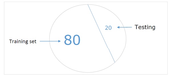
Hold-out dataset model ensures that we have enough data to train our ML model and at the same time we will have a reasonable number of samples to get good measurement of model’s performance.
In order to include in the training set and test set, it’s a good practice to choose random samples from the main dataset. It ensures an even distribution between training and test set.
Following is an example in which we are producing own hold-out dataset by using train_test_split function from the scikit-learn library.
Example
from sklearn.datasets import load_iris
iris = load_iris()
X = iris.data
y = iris.target
from sklearn.model_selection import train_test_split
X_train, X_test, y_train, y_test = train_test_split(X, y, test_size=0.2, random_state=1)
# Here above test_size = 0.2 represents that we provided 20% of the data as test data.
from sklearn.neighbors import KNeighborsClassifier
from sklearn import metrics
classifier_knn = KNeighborsClassifier(n_neighbors=3)
classifier_knn.fit(X_train, y_train)
y_pred = classifier_knn.predict(X_test)
# Providing sample data and the model will make prediction out of that data
sample = [[5, 5, 3, 2], [2, 4, 3, 5]]
preds = classifier_knn.predict(sample)
pred_species = [iris.target_names[p] for p in preds] print("Predictions:", pred_species)
Output
Predictions: ['versicolor', 'virginica']
While using CNTK, we need to randomise the order of our dataset each time we train our model because −
Deep learning algorithms are highly influenced by the random-number generators.
The order in which we provide the samples to NN during training greatly affects its performance.
The major downside of using the hold-out dataset technique is that it is unreliable because sometimes we get very good results but sometimes, we get bad results.
K-fold cross validation
To make our ML model more reliable, there is a technique called K-fold cross validation. In nature K-fold cross validation technique is same as the previous technique, but it repeats it several times-usually about 5 to 10 times. Following diagram represents its concept −
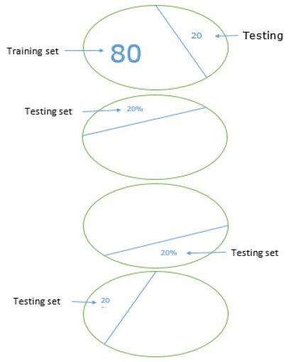
Working of K-fold cross validation
The working of K-fold cross validation can be understood with the help of following steps −
Step 1 − Like in Hand-out dataset technique, in K-fold cross validation technique, first we need to split the dataset into a training and test set. Ideally, the ratio is 80-20, i.e. 80% of training set and 20% of test set.
Step 2 − Next, we need to train our model using the training set.
Step 3 −At last, we will be using the test set to measure the performance of our model. The only difference between Hold-out dataset technique and k-cross validation technique is that the above process gets repeated usually for 5 to 10 times and at the end the average is calculated over all the performance metrics. That average would be the final performance metrics.
Let us see an example with a small dataset −
Example
from numpy import array
from sklearn.model_selection import KFold
data = array([0.1, 0.2, 0.3, 0.4, 0.5, 0.6, 0.7, 0.8, 0.9, 1.0])
kfold = KFold(5, True, 1)
for train, test in kfold.split(data):
   print('train: %s, test: %s' % (data[train],(data[test]))
Output
train: [0.1 0.2 0.4 0.5 0.6 0.7 0.8 0.9], test: [0.3 1. ]
train: [0.1 0.2 0.3 0.4 0.6 0.8 0.9 1. ], test: [0.5 0.7]
train: [0.2 0.3 0.5 0.6 0.7 0.8 0.9 1. ], test: [0.1 0.4]
train: [0.1 0.3 0.4 0.5 0.6 0.7 0.9 1. ], test: [0.2 0.8]
train: [0.1 0.2 0.3 0.4 0.5 0.7 0.8 1. ], test: [0.6 0.9]
As we see, because of using a more realistic training and test scenario, k-fold cross validation technique gives us a much more stable performance measurement but, on the downside, it takes a lot of time when validating deep learning models.
CNTK does not support for k-cross validation, hence we need to write our own script to do so.
Detecting underfitting and overfitting
Whether, we use Hand-out dataset or k-fold cross-validation technique, we will discover that the output for the metrics will be different for dataset used for training and the dataset used for validation.
Detecting overfitting
The phenomenon called overfitting is a situation where our ML model, models the training data exceptionally well, but fails to perform well on the testing data, i.e. was not able to predict test data.
It happens when a ML model learns a specific pattern and noise from the training data to such an extent, that it negatively impacts that model’s ability to generalise from the training data to new, i.e. unseen data. Here, noise is the irrelevant information or randomness in a dataset.
Following are the two ways with the help of which we can detect weather our model is overfit or not −
The overfit model will perform well on the same samples we used for training, but it will perform very bad on the new samples, i.e. samples different from training.
The model is overfit during validation if the metric on the test set is lower than the same metric, we use on our training set.
Detecting underfitting
Another situation that can arise in our ML is underfitting. This is a situation where, our ML model didn’t model the training data well and fails to predict useful output. When we start training the first epoch, our model will be underfitting, but will become less underfit as training progress.
One of the ways to detect, whether our model is underfit or not is to look at the metrics for training set and test set. Our model will be underfit if the metric on the test set is higher than the metric on the training set.
CNTK - Neural Network Classification
In this chapter, we will study how to classify neural network by using CNTK.
Introduction
Classification may be defined as the process to predict categorial output labels or responses for the given input data. The categorised output, which will be based on what the model has learned in training phase, can have the form such as "Black" or "White" or "spam" or "no spam".
On the other hand, mathematically, it is the task of approximating a mapping function say f from input variables say X to the output variables say Y.
A classic example of classification problem can be the spam detection in e-mails. It is obvious that there can be only two categories of output, "spam" and "no spam".
To implement such classification, we first need to do training of the classifier where "spam" and "no spam" emails would be used as the training data. Once, the classifier trained successfully, it can be used to detect an unknown email.
Here, we are going to create a 4-5-3 NN using iris flower dataset having the following −
4-input nodes (one for each predictor value).
5-hidden processing nodes.
3-output nodes (because there are three possible species in iris dataset).
Loading Dataset
We will be using iris flower dataset, from which we want to classify species of iris flowers based on the physical properties of sepal width and length, and petal width and length. The dataset describes the physical properties of different varieties of iris flowers −
Sepal length
Sepal width
Petal length
Petal width
Class i.e. iris setosa or iris versicolor or iris virginica
We have iris.CSV file which we used before in previous chapters also. It can be loaded with the help of Pandas library. But, before using it or loading it for our classifier, we need to prepare the training and test files, so that it can be used easily with CNTK.
Preparing training & test files
Iris dataset is one of the most popular datasets for ML projects. It has 150 data items and the raw data looks as follows −
5.1 3.5 1.4 0.2 setosa
4.9 3.0 1.4 0.2 setosa
…
7.0 3.2 4.7 1.4 versicolor
6.4 3.2 4.5 1.5 versicolor
…
6.3 3.3 6.0 2.5 virginica
5.8 2.7 5.1 1.9 virginica
As told earlier, the first four values on each line describes the physical properties of different varieties, i.e. Sepal length, Sepal width, Petal length, Petal width of iris flowers.
But, we should have to convert the data in the format, that can be easily used by CNTK and that format is .ctf file (we created one iris.ctf in previous section also). It will look like as follows −
|attribs 5.1 3.5 1.4 0.2|species 1 0 0
|attribs 4.9 3.0 1.4 0.2|species 1 0 0
…
|attribs 7.0 3.2 4.7 1.4|species 0 1 0
|attribs 6.4 3.2 4.5 1.5|species 0 1 0
…
|attribs 6.3 3.3 6.0 2.5|species 0 0 1
|attribs 5.8 2.7 5.1 1.9|species 0 0 1
In the above data, the |attribs tag mark the start of the feature value and the |species tags the class label values. We can also use any other tag names of our wish, even we can add item ID as well. For example, look at the following data −
|ID 001 |attribs 5.1 3.5 1.4 0.2|species 1 0 0 |#setosa
|ID 002 |attribs 4.9 3.0 1.4 0.2|species 1 0 0 |#setosa
…
|ID 051 |attribs 7.0 3.2 4.7 1.4|species 0 1 0 |#versicolor
|ID 052 |attribs 6.4 3.2 4.5 1.5|species 0 1 0 |#versicolor
…
There are total 150 data items in iris dataset and for this example, we will be using 80-20 hold-out dataset rule i.e. 80% (120 items) data items for training purpose and remaining 20% (30 items) data items for testing purpose.
Constructing Classification model
First, we need to process the data files in CNTK format and for that we are going to use the helper function named create_reader as follows −
def create_reader(path, input_dim, output_dim, rnd_order, sweeps):
x_strm = C.io.StreamDef(field='attribs', shape=input_dim, is_sparse=False)
y_strm = C.io.StreamDef(field='species', shape=output_dim, is_sparse=False)
streams = C.io.StreamDefs(x_src=x_strm, y_src=y_strm)
deserial = C.io.CTFDeserializer(path, streams)
mb_src = C.io.MinibatchSource(deserial, randomize=rnd_order, max_sweeps=sweeps)
return mb_src
Now, we need to set the architecture arguments for our NN and also provide the location of the data files. It can be done with the help of following python code −
def main():
print("Using CNTK version = " + str(C.__version__) + "\n")
input_dim = 4
hidden_dim = 5
output_dim = 3
train_file = ".\\...\\" #provide the name of the training file(120 data items)
test_file = ".\\...\\" #provide the name of the test file(30 data items)
Now, with the help of following code line our program will create the untrained NN −
X = C.ops.input_variable(input_dim, np.float32)
Y = C.ops.input_variable(output_dim, np.float32)
with C.layers.default_options(init=C.initializer.uniform(scale=0.01, seed=1)):
hLayer = C.layers.Dense(hidden_dim, activation=C.ops.tanh, name='hidLayer')(X)
oLayer = C.layers.Dense(output_dim, activation=None, name='outLayer')(hLayer)
nnet = oLayer
model = C.ops.softmax(nnet)
Now, once we created the dual untrained model, we need to set up a Learner algorithm object and afterwards use it to create a Trainer training object. We are going to use SGD learner and cross_entropy_with_softmax loss function −
tr_loss = C.cross_entropy_with_softmax(nnet, Y)
tr_clas = C.classification_error(nnet, Y)
max_iter = 2000
batch_size = 10
learn_rate = 0.01
learner = C.sgd(nnet.parameters, learn_rate)
trainer = C.Trainer(nnet, (tr_loss, tr_clas), [learner])
Code the learning algorithm as follows −
max_iter = 2000
batch_size = 10
lr_schedule = C.learning_parameter_schedule_per_sample([(1000, 0.05), (1, 0.01)])
mom_sch = C.momentum_schedule([(100, 0.99), (0, 0.95)], batch_size)
learner = C.fsadagrad(nnet.parameters, lr=lr_schedule, momentum=mom_sch)
trainer = C.Trainer(nnet, (tr_loss, tr_clas), [learner])
Now, once we finished with Trainer object, we need to create a reader function to read the training data−
rdr = create_reader(train_file, input_dim, output_dim, rnd_order=True, sweeps=C.io.INFINITELY_REPEAT)
iris_input_map = { X : rdr.streams.x_src, Y : rdr.streams.y_src }
Now it’s time to train our NN model−
for i in range(0, max_iter):
curr_batch = rdr.next_minibatch(batch_size, input_map=iris_input_map) trainer.train_minibatch(curr_batch)
if i % 500 == 0:
mcee = trainer.previous_minibatch_loss_average
macc = (1.0 - trainer.previous_minibatch_evaluation_average) * 100
print("batch %4d: mean loss = %0.4f, accuracy = %0.2f%% " \ % (i, mcee, macc))
Once, we have done with training, let’s evaluate the model using test data items −
print("\nEvaluating test data \n")
rdr = create_reader(test_file, input_dim, output_dim, rnd_order=False, sweeps=1)
iris_input_map = { X : rdr.streams.x_src, Y : rdr.streams.y_src }
num_test = 30
all_test = rdr.next_minibatch(num_test, input_map=iris_input_map) acc = (1.0 - trainer.test_minibatch(all_test)) * 100
print("Classification accuracy = %0.2f%%" % acc)
After evaluating the accuracy of our trained NN model, we will be using it for making a prediction on unseen data −
np.set_printoptions(precision = 1, suppress=True)
unknown = np.array([[6.4, 3.2, 4.5, 1.5]], dtype=np.float32)
print("\nPredicting Iris species for input features: ")
print(unknown[0]) pred_prob = model.eval(unknown)
np.set_printoptions(precision = 4, suppress=True)
print("Prediction probabilities are: ")
print(pred_prob[0])
Complete Classification Model
Import numpy as np
Import cntk as C
def create_reader(path, input_dim, output_dim, rnd_order, sweeps):
x_strm = C.io.StreamDef(field='attribs', shape=input_dim, is_sparse=False)
y_strm = C.io.StreamDef(field='species', shape=output_dim, is_sparse=False)
streams = C.io.StreamDefs(x_src=x_strm, y_src=y_strm)
deserial = C.io.CTFDeserializer(path, streams)
mb_src = C.io.MinibatchSource(deserial, randomize=rnd_order, max_sweeps=sweeps)
return mb_src
def main():
print("Using CNTK version = " + str(C.__version__) + "\n")
input_dim = 4
hidden_dim = 5
output_dim = 3
train_file = ".\\...\\" #provide the name of the training file(120 data items)
test_file = ".\\...\\" #provide the name of the test file(30 data items)
X = C.ops.input_variable(input_dim, np.float32)
Y = C.ops.input_variable(output_dim, np.float32)
with C.layers.default_options(init=C.initializer.uniform(scale=0.01, seed=1)):
hLayer = C.layers.Dense(hidden_dim, activation=C.ops.tanh, name='hidLayer')(X)
oLayer = C.layers.Dense(output_dim, activation=None, name='outLayer')(hLayer)
nnet = oLayer
model = C.ops.softmax(nnet)
tr_loss = C.cross_entropy_with_softmax(nnet, Y)
tr_clas = C.classification_error(nnet, Y)
max_iter = 2000
batch_size = 10
learn_rate = 0.01
learner = C.sgd(nnet.parameters, learn_rate)
trainer = C.Trainer(nnet, (tr_loss, tr_clas), [learner])
max_iter = 2000
batch_size = 10
lr_schedule = C.learning_parameter_schedule_per_sample([(1000, 0.05), (1, 0.01)])
mom_sch = C.momentum_schedule([(100, 0.99), (0, 0.95)], batch_size)
learner = C.fsadagrad(nnet.parameters, lr=lr_schedule, momentum=mom_sch)
trainer = C.Trainer(nnet, (tr_loss, tr_clas), [learner])
rdr = create_reader(train_file, input_dim, output_dim, rnd_order=True, sweeps=C.io.INFINITELY_REPEAT)
iris_input_map = { X : rdr.streams.x_src, Y : rdr.streams.y_src }
for i in range(0, max_iter):
curr_batch = rdr.next_minibatch(batch_size, input_map=iris_input_map) trainer.train_minibatch(curr_batch)
if i % 500 == 0:
mcee = trainer.previous_minibatch_loss_average
macc = (1.0 - trainer.previous_minibatch_evaluation_average) * 100
print("batch %4d: mean loss = %0.4f, accuracy = %0.2f%% " \ % (i, mcee, macc))
print("\nEvaluating test data \n")
rdr = create_reader(test_file, input_dim, output_dim, rnd_order=False, sweeps=1)
iris_input_map = { X : rdr.streams.x_src, Y : rdr.streams.y_src }
num_test = 30
all_test = rdr.next_minibatch(num_test, input_map=iris_input_map) acc = (1.0 - trainer.test_minibatch(all_test)) * 100
print("Classification accuracy = %0.2f%%" % acc)
np.set_printoptions(precision = 1, suppress=True)
unknown = np.array([[7.0, 3.2, 4.7, 1.4]], dtype=np.float32)
print("\nPredicting species for input features: ")
print(unknown[0])
pred_prob = model.eval(unknown)
np.set_printoptions(precision = 4, suppress=True)
print("Prediction probabilities: ")
print(pred_prob[0])
if __name__== ”__main__”:
main()
Output
Using CNTK version = 2.7
batch 0: mean loss = 1.0986, mean accuracy = 40.00%
batch 500: mean loss = 0.6677, mean accuracy = 80.00%
batch 1000: mean loss = 0.5332, mean accuracy = 70.00%
batch 1500: mean loss = 0.2408, mean accuracy = 100.00%
Evaluating test data
Classification accuracy = 94.58%
Predicting species for input features:
[7.0 3.2 4.7 1.4]
Prediction probabilities:
[0.0847 0.736 0.113]
Saving the trained model
This Iris dataset has only 150 data items, hence it would take only a few seconds to train the NN classifier model, but training on a large dataset having hundred or thousand data items can take hours or even days.
We can save our model so that, we won’t have to retain it from scratch. With the help of following Python code, we can save our trained NN −
nn_classifier = “.\\neuralclassifier.model” #provide the name of the file
model.save(nn_classifier, format=C.ModelFormat.CNTKv2)
Following are the arguments of save() function used above −
File name is the first argument of save() function. It can also be write along with the path of file.
Another parameter is the format parameter which has a default value C.ModelFormat.CNTKv2.
Loading the trained model
Once you saved the trained model, it’s very easy to load that model. We only need to use the load () function. Let’s check this in the following example −
import numpy as np
import cntk as C
model = C.ops.functions.Function.load(“.\\neuralclassifier.model”)
np.set_printoptions(precision = 1, suppress=True)
unknown = np.array([[7.0, 3.2, 4.7, 1.4]], dtype=np.float32)
print("\nPredicting species for input features: ")
print(unknown[0])
pred_prob = model.eval(unknown)
np.set_printoptions(precision = 4, suppress=True)
print("Prediction probabilities: ")
print(pred_prob[0])
The benefit of saved model is that, once you load a saved model, it can be used exactly as if the model had just been trained.
CNTK - Neural Network Binary Classification
Let us understand, what is neural network binary classification using CNTK, in this chapter.
Binary classification using NN is like multi-class classification, the only thing is that there are just two output nodes instead of three or more. Here, we are going to perform binary classification using a neural network by using two techniques namely one-node and two-node technique. One-node technique is more common than two-node technique.
Loading Dataset
For both these techniques to implement using NN, we will be using banknote dataset. The dataset can be downloaded from UCI Machine Learning Repository which is available at https://archive.ics.uci.edu/ml/datasets/banknote+authentication.
For our example, we will be using 50 authentic data items having class forgery = 0, and the first 50 fake items having class forgery = 1.
Preparing training & test files
There are 1372 data items in the full dataset. The raw dataset looks as follows −
3.6216, 8.6661, -2.8076, -0.44699, 0
4.5459, 8.1674, -2.4586, -1.4621, 0
…
-1.3971, 3.3191, -1.3927, -1.9948, 1
0.39012, -0.14279, -0.031994, 0.35084, 1
Now, first we need to convert this raw data into two-node CNTK format, which would be as follows −
|stats 3.62160000 8.66610000 -2.80730000 -0.44699000 |forgery 0 1 |# authentic
|stats 4.54590000 8.16740000 -2.45860000 -1.46210000 |forgery 0 1 |# authentic
. . .
|stats -1.39710000 3.31910000 -1.39270000 -1.99480000 |forgery 1 0 |# fake
|stats 0.39012000 -0.14279000 -0.03199400 0.35084000 |forgery 1 0 |# fake
You can use the following python program to create CNTK-format data from Raw data −
fin = open(".\\...", "r") #provide the location of saved dataset text file.
for line in fin:
   line = line.strip()
   tokens = line.split(",")
   if tokens[4] == "0":
    print("|stats %12.8f %12.8f %12.8f %12.8f |forgery 0 1 |# authentic" % \
(float(tokens[0]), float(tokens[1]), float(tokens[2]), float(tokens[3])) )
   else:
    print("|stats %12.8f %12.8f %12.8f %12.8f |forgery 1 0 |# fake" % \
(float(tokens[0]), float(tokens[1]), float(tokens[2]), float(tokens[3])) )
fin.close()
Two-node binary Classification model
There is very little difference between two-node classification and multi-class classification. Here we first, need to process the data files in CNTK format and for that we are going to use the helper function named create_reader as follows −
def create_reader(path, input_dim, output_dim, rnd_order, sweeps):
x_strm = C.io.StreamDef(field='stats', shape=input_dim, is_sparse=False)
y_strm = C.io.StreamDef(field='forgery', shape=output_dim, is_sparse=False)
streams = C.io.StreamDefs(x_src=x_strm, y_src=y_strm)
deserial = C.io.CTFDeserializer(path, streams)
mb_src = C.io.MinibatchSource(deserial, randomize=rnd_order, max_sweeps=sweeps)
return mb_src
Now, we need to set the architecture arguments for our NN and also provide the location of the data files. It can be done with the help of following python code −
def main():
print("Using CNTK version = " + str(C.__version__) + "\n")
input_dim = 4
hidden_dim = 10
output_dim = 2
train_file = ".\\...\\" #provide the name of the training file
test_file = ".\\...\\" #provide the name of the test file
Now, with the help of following code line our program will create the untrained NN −
X = C.ops.input_variable(input_dim, np.float32)
Y = C.ops.input_variable(output_dim, np.float32)
with C.layers.default_options(init=C.initializer.uniform(scale=0.01, seed=1)):
hLayer = C.layers.Dense(hidden_dim, activation=C.ops.tanh, name='hidLayer')(X)
oLayer = C.layers.Dense(output_dim, activation=None, name='outLayer')(hLayer)
nnet = oLayer
model = C.ops.softmax(nnet)
Now, once we created the dual untrained model, we need to set up a Learner algorithm object and afterwards use it to create a Trainer training object. We are going to use SGD learner and cross_entropy_with_softmax loss function −
tr_loss = C.cross_entropy_with_softmax(nnet, Y)
tr_clas = C.classification_error(nnet, Y)
max_iter = 500
batch_size = 10
learn_rate = 0.01
learner = C.sgd(nnet.parameters, learn_rate)
trainer = C.Trainer(nnet, (tr_loss, tr_clas), [learner])
Now, once we finished with Trainer object, we need to create a reader function to read the training data −
rdr = create_reader(train_file, input_dim, output_dim, rnd_order=True, sweeps=C.io.INFINITELY_REPEAT)
banknote_input_map = { X : rdr.streams.x_src, Y : rdr.streams.y_src }
Now, it is time to train our NN model −
for i in range(0, max_iter):
curr_batch = rdr.next_minibatch(batch_size, input_map=iris_input_map) trainer.train_minibatch(curr_batch)
if i % 500 == 0:
mcee = trainer.previous_minibatch_loss_average
macc = (1.0 - trainer.previous_minibatch_evaluation_average) * 100
print("batch %4d: mean loss = %0.4f, accuracy = %0.2f%% " \ % (i, mcee, macc))
Once training is completed, let us evaluate the model using test data items −
print("\nEvaluating test data \n")
rdr = create_reader(test_file, input_dim, output_dim, rnd_order=False, sweeps=1)
banknote_input_map = { X : rdr.streams.x_src, Y : rdr.streams.y_src }
num_test = 20
all_test = rdr.next_minibatch(num_test, input_map=iris_input_map) acc = (1.0 - trainer.test_minibatch(all_test)) * 100
print("Classification accuracy = %0.2f%%" % acc)
After evaluating the accuracy of our trained NN model, we will be using it for making a prediction on unseen data −
np.set_printoptions(precision = 1, suppress=True)
unknown = np.array([[0.6, 1.9, -3.3, -0.3]], dtype=np.float32)
print("\nPredicting Banknote authenticity for input features: ")
print(unknown[0])
pred_prob = model.eval(unknown)
np.set_printoptions(precision = 4, suppress=True)
print("Prediction probabilities are: ")
print(pred_prob[0])
if pred_prob[0,0] < pred_prob[0,1]:
  print(“Prediction: authentic”)
else:
  print(“Prediction: fake”)
Complete Two-node Classification Model
def create_reader(path, input_dim, output_dim, rnd_order, sweeps):
x_strm = C.io.StreamDef(field='stats', shape=input_dim, is_sparse=False)
y_strm = C.io.StreamDef(field='forgery', shape=output_dim, is_sparse=False)
streams = C.io.StreamDefs(x_src=x_strm, y_src=y_strm)
deserial = C.io.CTFDeserializer(path, streams)
mb_src = C.io.MinibatchSource(deserial, randomize=rnd_order, max_sweeps=sweeps)
return mb_src
def main():
print("Using CNTK version = " + str(C.__version__) + "\n")
input_dim = 4
hidden_dim = 10
output_dim = 2
train_file = ".\\...\\" #provide the name of the training file
test_file = ".\\...\\" #provide the name of the test file
X = C.ops.input_variable(input_dim, np.float32)
Y = C.ops.input_variable(output_dim, np.float32)
withC.layers.default_options(init=C.initializer.uniform(scale=0.01, seed=1)):
hLayer = C.layers.Dense(hidden_dim, activation=C.ops.tanh, name='hidLayer')(X)
oLayer = C.layers.Dense(output_dim, activation=None, name='outLayer')(hLayer)
nnet = oLayer
model = C.ops.softmax(nnet)
tr_loss = C.cross_entropy_with_softmax(nnet, Y)
tr_clas = C.classification_error(nnet, Y)
max_iter = 500
batch_size = 10
learn_rate = 0.01
learner = C.sgd(nnet.parameters, learn_rate)
trainer = C.Trainer(nnet, (tr_loss, tr_clas), [learner])
rdr = create_reader(train_file, input_dim, output_dim, rnd_order=True, sweeps=C.io.INFINITELY_REPEAT)
banknote_input_map = { X : rdr.streams.x_src, Y : rdr.streams.y_src }
for i in range(0, max_iter):
curr_batch = rdr.next_minibatch(batch_size, input_map=iris_input_map) trainer.train_minibatch(curr_batch)
if i % 500 == 0:
mcee = trainer.previous_minibatch_loss_average
macc = (1.0 - trainer.previous_minibatch_evaluation_average) * 100
print("batch %4d: mean loss = %0.4f, accuracy = %0.2f%% " \ % (i, mcee, macc))
print("\nEvaluating test data \n")
rdr = create_reader(test_file, input_dim, output_dim, rnd_order=False, sweeps=1)
banknote_input_map = { X : rdr.streams.x_src, Y : rdr.streams.y_src }
num_test = 20
all_test = rdr.next_minibatch(num_test, input_map=iris_input_map) acc = (1.0 - trainer.test_minibatch(all_test)) * 100
print("Classification accuracy = %0.2f%%" % acc)
np.set_printoptions(precision = 1, suppress=True)
unknown = np.array([[0.6, 1.9, -3.3, -0.3]], dtype=np.float32)
print("\nPredicting Banknote authenticity for input features: ")
print(unknown[0])
pred_prob = model.eval(unknown)
np.set_printoptions(precision = 4, suppress=True)
print("Prediction probabilities are: ")
print(pred_prob[0])
if pred_prob[0,0] < pred_prob[0,1]:
print(“Prediction: authentic”)
else:
print(“Prediction: fake”)
if __name__== ”__main__”:
main()
Output
Using CNTK version = 2.7
batch 0: mean loss = 0.6928, accuracy = 80.00%
batch 50: mean loss = 0.6877, accuracy = 70.00%
batch 100: mean loss = 0.6432, accuracy = 80.00%
batch 150: mean loss = 0.4978, accuracy = 80.00%
batch 200: mean loss = 0.4551, accuracy = 90.00%
batch 250: mean loss = 0.3755, accuracy = 90.00%
batch 300: mean loss = 0.2295, accuracy = 100.00%
batch 350: mean loss = 0.1542, accuracy = 100.00%
batch 400: mean loss = 0.1581, accuracy = 100.00%
batch 450: mean loss = 0.1499, accuracy = 100.00%
Evaluating test data
Classification accuracy = 84.58%
Predicting banknote authenticity for input features:
[0.6 1.9 -3.3 -0.3]
Prediction probabilities are:
[0.7847 0.2536]
Prediction: fake
One-node binary Classification model
The implementation program is almost like we have done above for two-node classification. The main change is that when using the two-node classification technique.
We can use the CNTK built-in classification_error() function, but in case of one-node classification CNTK doesn’t support classification_error() function. That’s the reason we need to implement a program-defined function as follows −
def class_acc(mb, x_var, y_var, model):
num_correct = 0; num_wrong = 0
x_mat = mb[x_var].asarray()
y_mat = mb[y_var].asarray()
for i in range(mb[x_var].shape[0]):
   p = model.eval(x_mat[i]
   y = y_mat[i]
   if p[0,0] < 0.5 and y[0,0] == 0.0 or p[0,0] >= 0.5 and y[0,0] == 1.0:
num_correct += 1
 else:
  num_wrong += 1
return (num_correct * 100.0)/(num_correct + num_wrong)
With that change let’s see the complete one-node classification example −
Complete one-node Classification Model
import numpy as np
import cntk as C
def create_reader(path, input_dim, output_dim, rnd_order, sweeps):
x_strm = C.io.StreamDef(field='stats', shape=input_dim, is_sparse=False)
y_strm = C.io.StreamDef(field='forgery', shape=output_dim, is_sparse=False)
streams = C.io.StreamDefs(x_src=x_strm, y_src=y_strm)
deserial = C.io.CTFDeserializer(path, streams)
mb_src = C.io.MinibatchSource(deserial, randomize=rnd_order, max_sweeps=sweeps)
return mb_src
def class_acc(mb, x_var, y_var, model):
num_correct = 0; num_wrong = 0
x_mat = mb[x_var].asarray()
y_mat = mb[y_var].asarray()
for i in range(mb[x_var].shape[0]):
  p = model.eval(x_mat[i]
  y = y_mat[i]
  if p[0,0] < 0.5 and y[0,0] == 0.0 or p[0,0] >= 0.5 and y[0,0] == 1.0:
  num_correct += 1
 else:
  num_wrong += 1
return (num_correct * 100.0)/(num_correct + num_wrong)
def main():
print("Using CNTK version = " + str(C.__version__) + "\n")
input_dim = 4
hidden_dim = 10
output_dim = 1
train_file = ".\\...\\" #provide the name of the training file
test_file = ".\\...\\" #provide the name of the test file
X = C.ops.input_variable(input_dim, np.float32)
Y = C.ops.input_variable(output_dim, np.float32)
with C.layers.default_options(init=C.initializer.uniform(scale=0.01, seed=1)):
hLayer = C.layers.Dense(hidden_dim, activation=C.ops.tanh, name='hidLayer')(X)
oLayer = C.layers.Dense(output_dim, activation=None, name='outLayer')(hLayer)
model = oLayer
tr_loss = C.cross_entropy_with_softmax(model, Y)
max_iter = 1000
batch_size = 10
learn_rate = 0.01
learner = C.sgd(model.parameters, learn_rate)
trainer = C.Trainer(model, (tr_loss), [learner])
rdr = create_reader(train_file, input_dim, output_dim, rnd_order=True, sweeps=C.io.INFINITELY_REPEAT)
banknote_input_map = {X : rdr.streams.x_src, Y : rdr.streams.y_src }
for i in range(0, max_iter):
curr_batch = rdr.next_minibatch(batch_size, input_map=iris_input_map) trainer.train_minibatch(curr_batch)
if i % 100 == 0:
mcee=trainer.previous_minibatch_loss_average
ca = class_acc(curr_batch, X,Y, model)
print("batch %4d: mean loss = %0.4f, accuracy = %0.2f%% " \ % (i, mcee, ca))
print("\nEvaluating test data \n")
rdr = create_reader(test_file, input_dim, output_dim, rnd_order=False, sweeps=1)
banknote_input_map = { X : rdr.streams.x_src, Y : rdr.streams.y_src }
num_test = 20
all_test = rdr.next_minibatch(num_test, input_map=iris_input_map)
acc = class_acc(all_test, X,Y, model)
print("Classification accuracy = %0.2f%%" % acc)
np.set_printoptions(precision = 1, suppress=True)
unknown = np.array([[0.6, 1.9, -3.3, -0.3]], dtype=np.float32)
print("\nPredicting Banknote authenticity for input features: ")
print(unknown[0])
pred_prob = model.eval({X:unknown})
print("Prediction probability: ")
print(“%0.4f” % pred_prob[0,0])
if pred_prob[0,0] < 0.5:
  print(“Prediction: authentic”)
else:
  print(“Prediction: fake”)
if __name__== ”__main__”:
   main()
Output
Using CNTK version = 2.7
batch 0: mean loss = 0.6936, accuracy = 10.00%
batch 100: mean loss = 0.6882, accuracy = 70.00%
batch 200: mean loss = 0.6597, accuracy = 50.00%
batch 300: mean loss = 0.5298, accuracy = 70.00%
batch 400: mean loss = 0.4090, accuracy = 100.00%
batch 500: mean loss = 0.3790, accuracy = 90.00%
batch 600: mean loss = 0.1852, accuracy = 100.00%
batch 700: mean loss = 0.1135, accuracy = 100.00%
batch 800: mean loss = 0.1285, accuracy = 100.00%
batch 900: mean loss = 0.1054, accuracy = 100.00%
Evaluating test data
Classification accuracy = 84.00%
Predicting banknote authenticity for input features:
[0.6 1.9 -3.3 -0.3]
Prediction probability:
0.8846
Prediction: fake
CNTK - Neural Network Regression
The chapter will help you understand the neural network regression with regards to CNTK.
Introduction
As we know that, in order to predict a numeric value from one or more predictor variables, we use regression. Let’s take an example of predicting the median value of a house in say one of the 100 towns. To do so, we have data that includes −
A crime statistic for each town.
The age of the houses in each town.
A measure of the distance from each town to a prime location.
The student-to-teacher ratio in each town.
A racial demographic statistic for each town.
The median house value in each town.
Based on these five predictor variables, we would like to predict median house value. And for this we can create a linear regression model along the lines of−
Y = a0+a1(crime)+a2(house-age)+(a3)(distance)+(a4)(ratio)+(a5)(racial)
In the above equation −
Y is a predicted median value
a0 is a constant and
a1 through a5 all are constants associated with the five predictors we discussed above.
We also have an alternate approach of using a neural network. It will create more accurate prediction model.
Here, we will be creating a neural network regression model by using CNTK.
Loading Dataset
To implement Neural Network regression using CNTK, we will be using Boston area house values dataset. The dataset can be downloaded from UCI Machine Learning Repository which is available at https://archive.ics.uci.edu/. This dataset has total 14 variables and 506 instances.
But, for our implementation program we are going to use six of the 14 variables and 100 instances. Out of 6, 5 as predictors and one as a value-to-predict. From 100 instances, we will be using 80 for training and 20 for testing purpose. The value which we want to predict is the median house price in a town. Let’s see the five predictors we will be using −
Crime per capita in the town − We would expect smaller values to be associated with this predictor.
Proportion of owner − occupied units built before 1940 - We would expect smaller values to be associated with this predictor because larger value means older house.
Weighed distance of the town to five Boston employment centers.
Area school pupil-to-teacher ratio.
An indirect metric of the proportion of black residents in the town.
Preparing training & test files
As we did before, first we need to convert the raw data into CNTK format. We are going to use first 80 data items for training purpose, so the tab-delimited CNTK format is as follows −
|predictors 1.612820 96.90 3.76 21.00 248.31 |medval 13.50
|predictors 0.064170 68.20 3.36 19.20 396.90 |medval 18.90
|predictors 0.097440 61.40 3.38 19.20 377.56 |medval 20.00
. . .
Next 20 items, also converted into CNTK format, will used for testing purpose.
Constructing Regression model
First, we need to process the data files in CNTK format and for that, we are going to use the helper function named create_reader as follows −
def create_reader(path, input_dim, output_dim, rnd_order, sweeps):
x_strm = C.io.StreamDef(field='predictors', shape=input_dim, is_sparse=False)
y_strm = C.io.StreamDef(field='medval', shape=output_dim, is_sparse=False)
streams = C.io.StreamDefs(x_src=x_strm, y_src=y_strm)
deserial = C.io.CTFDeserializer(path, streams)
mb_src = C.io.MinibatchSource(deserial, randomize=rnd_order, max_sweeps=sweeps)
return mb_src
Next, we need to create a helper function that accepts a CNTK mini-batch object and computes a custom accuracy metric.
def mb_accuracy(mb, x_var, y_var, model, delta):
   num_correct = 0
   num_wrong = 0
   x_mat = mb[x_var].asarray()
   y_mat = mb[y_var].asarray()
for i in range(mb[x_var].shape[0]):
  v = model.eval(x_mat[i])
  y = y_mat[i]
if np.abs(v[0,0] – y[0,0]) < delta:
   num_correct += 1
else:
   num_wrong += 1
return (num_correct * 100.0)/(num_correct + num_wrong)
Now, we need to set the architecture arguments for our NN and also provide the location of the data files. It can be done with the help of following python code −
def main():
print("Using CNTK version = " + str(C.__version__) + "\n")
input_dim = 5
hidden_dim = 20
output_dim = 1
train_file = ".\\...\\" #provide the name of the training file(80 data items)
test_file = ".\\...\\" #provide the name of the test file(20 data items)
Now, with the help of following code line our program will create the untrained NN −
X = C.ops.input_variable(input_dim, np.float32)
Y = C.ops.input_variable(output_dim, np.float32)
with C.layers.default_options(init=C.initializer.uniform(scale=0.01, seed=1)):
hLayer = C.layers.Dense(hidden_dim, activation=C.ops.tanh, name='hidLayer')(X)
oLayer = C.layers.Dense(output_dim, activation=None, name='outLayer')(hLayer)
model = C.ops.alias(oLayer)
Now, once we have created the dual untrained model, we need to set up a Learner algorithm object. We are going to use SGD learner and squared_error loss function −
tr_loss = C.squared_error(model, Y)
max_iter = 3000
batch_size = 5
base_learn_rate = 0.02
sch=C.learning_parameter_schedule([base_learn_rate, base_learn_rate/2], minibatch_size=batch_size, epoch_size=int((max_iter*batch_size)/2))
learner = C.sgd(model.parameters, sch)
trainer = C.Trainer(model, (tr_loss), [learner])
Now, once we finish with Learning algorithm object, we need to create a reader function to read the training data −
rdr = create_reader(train_file, input_dim, output_dim, rnd_order=True, sweeps=C.io.INFINITELY_REPEAT)
boston_input_map = { X : rdr.streams.x_src, Y : rdr.streams.y_src }
Now, it’s time to train our NN model −
for i in range(0, max_iter):
curr_batch = rdr.next_minibatch(batch_size, input_map=boston_input_map) trainer.train_minibatch(curr_batch)
if i % int(max_iter/10) == 0:
mcee = trainer.previous_minibatch_loss_average
acc = mb_accuracy(curr_batch, X, Y, model, delta=3.00)
print("batch %4d: mean squared error = %8.4f, accuracy = %5.2f%% " \ % (i, mcee, acc))
Once we have done with training, let’s evaluate the model using test data items −
print("\nEvaluating test data \n")
rdr = create_reader(test_file, input_dim, output_dim, rnd_order=False, sweeps=1)
boston_input_map = { X : rdr.streams.x_src, Y : rdr.streams.y_src }
num_test = 20
all_test = rdr.next_minibatch(num_test, input_map=boston_input_map)
acc = mb_accuracy(all_test, X, Y, model, delta=3.00)
print("Prediction accuracy = %0.2f%%" % acc)
After evaluating the accuracy of our trained NN model, we will be using it for making a prediction on unseen data −
np.set_printoptions(precision = 2, suppress=True)
unknown = np.array([[0.09, 50.00, 4.5, 17.00, 350.00], dtype=np.float32)
print("\nPredicting median home value for feature/predictor values: ")
print(unknown[0])
pred_prob = model.eval({X: unknown)
print("\nPredicted value is: ")
print(“$%0.2f (x1000)” %pred_value[0,0])
Complete Regression Model
import numpy as np
import cntk as C
def create_reader(path, input_dim, output_dim, rnd_order, sweeps):
x_strm = C.io.StreamDef(field='predictors', shape=input_dim, is_sparse=False)
y_strm = C.io.StreamDef(field='medval', shape=output_dim, is_sparse=False)
streams = C.io.StreamDefs(x_src=x_strm, y_src=y_strm)
deserial = C.io.CTFDeserializer(path, streams)
mb_src = C.io.MinibatchSource(deserial, randomize=rnd_order, max_sweeps=sweeps)
return mb_src
def mb_accuracy(mb, x_var, y_var, model, delta):
num_correct = 0
num_wrong = 0
x_mat = mb[x_var].asarray()
y_mat = mb[y_var].asarray()
for i in range(mb[x_var].shape[0]):
   v = model.eval(x_mat[i])
   y = y_mat[i]
if np.abs(v[0,0] – y[0,0]) < delta:
   num_correct += 1
else:
   num_wrong += 1
return (num_correct * 100.0)/(num_correct + num_wrong)
def main():
print("Using CNTK version = " + str(C.__version__) + "\n")
input_dim = 5
hidden_dim = 20
output_dim = 1
train_file = ".\\...\\" #provide the name of the training file(80 data items)
test_file = ".\\...\\" #provide the name of the test file(20 data items)
X = C.ops.input_variable(input_dim, np.float32)
Y = C.ops.input_variable(output_dim, np.float32)
with C.layers.default_options(init=C.initializer.uniform(scale=0.01, seed=1)):
hLayer = C.layers.Dense(hidden_dim, activation=C.ops.tanh, name='hidLayer')(X)
oLayer = C.layers.Dense(output_dim, activation=None, name='outLayer')(hLayer)
model = C.ops.alias(oLayer)
tr_loss = C.squared_error(model, Y)
max_iter = 3000
batch_size = 5
base_learn_rate = 0.02
sch = C.learning_parameter_schedule([base_learn_rate, base_learn_rate/2], minibatch_size=batch_size, epoch_size=int((max_iter*batch_size)/2))
learner = C.sgd(model.parameters, sch)
trainer = C.Trainer(model, (tr_loss), [learner])
rdr = create_reader(train_file, input_dim, output_dim, rnd_order=True, sweeps=C.io.INFINITELY_REPEAT)
boston_input_map = { X : rdr.streams.x_src, Y : rdr.streams.y_src }
for i in range(0, max_iter):
curr_batch = rdr.next_minibatch(batch_size, input_map=boston_input_map) trainer.train_minibatch(curr_batch)
if i % int(max_iter/10) == 0:
   mcee = trainer.previous_minibatch_loss_average
   acc = mb_accuracy(curr_batch, X, Y, model, delta=3.00)
   print("batch %4d: mean squared error = %8.4f, accuracy = %5.2f%% " \ % (i, mcee, acc))
   print("\nEvaluating test data \n")
   rdr = create_reader(test_file, input_dim, output_dim, rnd_order=False, sweeps=1)
   boston_input_map = { X : rdr.streams.x_src, Y : rdr.streams.y_src }
   num_test = 20
all_test = rdr.next_minibatch(num_test, input_map=boston_input_map)
acc = mb_accuracy(all_test, X, Y, model, delta=3.00)
print("Prediction accuracy = %0.2f%%" % acc)
np.set_printoptions(precision = 2, suppress=True)
unknown = np.array([[0.09, 50.00, 4.5, 17.00, 350.00], dtype=np.float32)
print("\nPredicting median home value for feature/predictor values: ")
print(unknown[0])
pred_prob = model.eval({X: unknown)
print("\nPredicted value is: ")
print(“$%0.2f (x1000)” %pred_value[0,0])
if __name__== ”__main__”:
   main()
Output
Using CNTK version = 2.7
batch 0: mean squared error = 385.6727, accuracy = 0.00%
batch 300: mean squared error = 41.6229, accuracy = 20.00%
batch 600: mean squared error = 28.7667, accuracy = 40.00%
batch 900: mean squared error = 48.6435, accuracy = 40.00%
batch 1200: mean squared error = 77.9562, accuracy = 80.00%
batch 1500: mean squared error = 7.8342, accuracy = 60.00%
batch 1800: mean squared error = 47.7062, accuracy = 60.00%
batch 2100: mean squared error = 40.5068, accuracy = 40.00%
batch 2400: mean squared error = 46.5023, accuracy = 40.00%
batch 2700: mean squared error = 15.6235, accuracy = 60.00%
Evaluating test data
Prediction accuracy = 64.00%
Predicting median home value for feature/predictor values:
[0.09 50. 4.5 17. 350.]
Predicted value is:
$21.02(x1000)
Saving the trained model
This Boston Home value dataset has only 506 data items (among which we sued only 100). Hence, it would take only a few seconds to train the NN regressor model, but training on a large dataset having hundred or thousand data items can take hours or even days.
We can save our model, so that we won’t have to retain it from scratch. With the help of following Python code, we can save our trained NN −
nn_regressor = “.\\neuralregressor.model” #provide the name of the file
model.save(nn_regressor, format=C.ModelFormat.CNTKv2)
Following are the arguments of save() function used above −
File name is the first argument of save() function. It can also be written along with the path of file.
Another parameter is the format parameter which has a default value C.ModelFormat.CNTKv2.
Loading the trained model
Once you saved the trained model, it’s very easy to load that model. We only need to use the load () function. Let’s check this in following example −
import numpy as np
import cntk as C
model = C.ops.functions.Function.load(“.\\neuralregressor.model”)
np.set_printoptions(precision = 2, suppress=True)
unknown = np.array([[0.09, 50.00, 4.5, 17.00, 350.00], dtype=np.float32)
print("\nPredicting area median home value for feature/predictor values: ")
print(unknown[0])
pred_prob = model.eval({X: unknown)
print("\nPredicted value is: ")
print(“$%0.2f (x1000)” %pred_value[0,0])
The benefit of saved model is that once you load a saved model, it can be used exactly as if the model had just been trained.
CNTK - Classification Model
This chapter will help you to understand how to measure performance of classification model in CNTK. Let us begin with confusion matrix.
Confusion matrix
Confusion matrix - a table with the predicted output versus the expected output is the easiest way to measure the performance of a classification problem, where the output can be of two or more type of classes.
In order to understand how it works, we are going to create a confusion matrix for a binary classification model that predicts, whether a credit card transaction was normal or a fraud. It is shown as follows −
| Actual fraud | Actual normal | |
|---|---|---|
|
Predicted fraud |
True positive |
False positive |
|
Predicted normal |
False negative |
True negative |
As we can see, the above sample confusion matrix contains 2 columns, one for class fraud and other for class normal. In the same way we have 2 rows, one is added for class fraud and other is added for class normal. Following is the explanation of the terms associated with confusion matrix −
True Positives − When both actual class & predicted class of data point is 1.
True Negatives − When both actual class & predicted class of data point is 0.
False Positives − When actual class of data point is 0 & predicted class of data point is 1.
False Negatives − When actual class of data point is 1 & predicted class of data point is 0.
Let’s see, how we can calculate number of different things from the confusion matrix −
Accuracy − It is the number of correct predictions made by our ML classification model. It can be calculated with the help of following formula −
Precision −It tells us how many samples were correctly predicted out of all samples we predicted. It can be calculated with the help of following formula −
Recall or Sensitivity − Recall are the number of positives returned by our ML classification model. In other words, it tells us how many of the fraud cases in the dataset were actually detected by the model. It can be calculated with the help of following formula −
Specificity − Opposite to recall, it gives the number of negatives returned by our ML classification model. It can be calculated with the help of following formula −
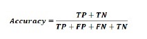
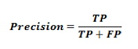
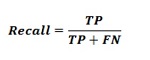
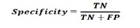
F-measure
We can use F-measure as an alternative of Confusion matrix. The main reason behind this, we can’t maximize Recall and Precision at the same time. There is a very strong relationship between these metrics and that can be understood with the help of following example −
Suppose, we want to use a DL model to classify cell samples as cancerous or normal. Here, to reach maximum precision we need to reduce the number of predictions to 1. Although, this can give us reach around 100 percent precision, but recall will become really low.
On the other hand, if we would like to reach maximum recall, we need to make as many predictions as possible. Although, this can give us reach around 100 percent recall, but precision will become really low.
In practice, we need to find a way balancing between precision and recall. The F-measure metric allows us to do so, as it expresses a harmonic average between precision and recall.
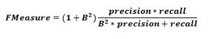
This formula is called the F1-measure, where the extra term called B is set to 1 to get an equal ratio of precision and recall. In order to emphasize recall, we can set the factor B to 2. On the other hand, to emphasize precision, we can set the factor B to 0.5.
Using CNTK to measure classification performance
In previous section we have created a classification model using Iris flower dataset. Here, we will be measuring its performance by using confusion matrix and F-measure metric.
Creating Confusion matrix
We already created the model, so we can start the validating process, which includes confusion matrix, on the same. First, we are going to create confusion matrix with the help of the confusion_matrix function from scikit-learn. For this, we need the real labels for our test samples and the predicted labels for the same test samples.
Let’s calculate the confusion matrix by using following python code −
from sklearn.metrics import confusion_matrix
y_true = np.argmax(y_test, axis=1)
y_pred = np.argmax(z(X_test), axis=1)
matrix = confusion_matrix(y_true=y_true, y_pred=y_pred)
print(matrix)
Output
[[10 0 0]
[ 0 1 9]
[ 0 0 10]]
We can also use heatmap function to visualise a confusion matrix as follows −
import seaborn as sns
import matplotlib.pyplot as plt
g = sns.heatmap(matrix,
     annot=True,
     xticklabels=label_encoder.classes_.tolist(),
     yticklabels=label_encoder.classes_.tolist(),
     cmap='Blues')
g.set_yticklabels(g.get_yticklabels(), rotation=0)
plt.show()
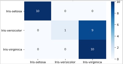
We should also have a single performance number, that we can use to compare the model. For this, we need to calculate the classification error by using classification_error function, from the metrics package in CNTK as done while creating classification model.
Now to calculate the classification error, execute the test method on the loss function with a dataset. After that, CNTK will take the samples we provided as input for this function and make a prediction based on input features X_test.
loss.test([X_test, y_test])
Output
{'metric': 0.36666666666, 'samples': 30}
Implementing F-Measures
For implementing F-Measures, CNTK also includes function called fmeasures. We can use this function, while training the NN by replacing the cell cntk.metrics.classification_error, with a call to cntk.losses.fmeasure when defining the criterion factory function as follows −
import cntk
@cntk.Function
def criterion_factory(output, target):
   loss = cntk.losses.cross_entropy_with_softmax(output, target)
metric = cntk.losses.fmeasure(output, target)
   return loss, metric
After using cntk.losses.fmeasure function, we will get different output for the loss.test method call given as follows −
loss.test([X_test, y_test])
Output
{'metric': 0.83101488749, 'samples': 30}
CNTK - Regression Model
Here, we will study about measuring performance with regards to a regression model.
Basics of validating a regression model
As we know that regression models are different than classification models, in the sense that, there is no binary measure of right or wrong for individuals’ samples. In regression models, we want to measure how close the prediction is to the actual value. The closer the prediction value is to the expected output, the better the model performs.
Here, we are going to measure the performance of NN used for regression using different error-rate functions.
Calculating error margin
As discussed earlier, while validating a regression model, we can’t say whether a prediction is right or wrong. We want our prediction to be as close as possible to the real value. But, a small error margin is acceptable here.
The formula for calculating the error margin is as follows −
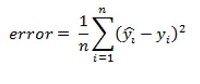
Here,
Predicted value = indicated y by a hat
Real value = predicted by y
First, we need to calculate the distance between the predicted and the real value. Then, to get an overall error rate, we need to sum these squared distances and calculate the average. This is called the mean squared error function.
But, if we want performance figures that express an error margin, we need a formula that expresses the absolute error. The formula for mean absolute error function is as follows −
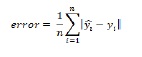
The above formula takes the absolute distance between the predicted and the real value.
Using CNTK to measure regression performance
Here, we will look at how to use the different metrics, we discussed in combination with CNTK. We will use a regression model, that predicts miles per gallon for cars using the steps given below.
Implementation steps−
Step 1 − First, we need to import the required components from cntk package as follows −
from cntk import default_option, input_variable
from cntk.layers import Dense, Sequential
from cntk.ops import relu
Step 2 − Next, we need to define a default activation function using the default_options functions. Then, create a new Sequential layer set and provide two Dense layers with 64 neurons each. Then, we add an additional Dense layer (which will act as the output layer) to the Sequential layer set and give 1 neuron without an activation as follows −
with default_options(activation=relu):
model = Sequential([Dense(64),Dense(64),Dense(1,activation=None)])
Step 3 − Once the network has been created, we need to create an input feature. We need to make sure that, it has the same shape as the features that we are going to be using for training.
features = input_variable(X.shape[1])
Step 4 − Now, we need to create another input_variable with size 1. It will be used to store the expected value for NN.
target = input_variable(1)
z = model(features)
Now, we need to train the model and in order to do so, we are going to split the dataset and perform preprocessing using the following implementation steps −
Step 5 −First, import StandardScaler from sklearn.preprocessing to get the values between -1 and +1. This will help us against exploding gradient problems in the NN.
from sklearn.preprocessing import StandardScalar
Step 6 − Next, import train_test_split from sklearn.model_selection as follows−
from sklearn.model_selection import train_test_split
Step 7 − Drop the mpg column from the dataset by using the dropmethod. At last split the dataset into a training and validation set using the train_test_split function as follows −
x = df_cars.drop(columns=[‘mpg’]).values.astype(np.float32)
y=df_cars.iloc[: , 0].values.reshape(-1, 1).astype(np.float32)
scaler = StandardScaler()
X = scaler.fit_transform(x)
X_train, X_test, y_train, y_test = train_test_split(X, y, test_size=0.2)
Step 8 − Now, we need to create another input_variable with size 1. It will be used to store the expected value for NN.
target = input_variable(1)
z = model(features)
We have split as well as preprocessed the data, now we need to train the NN. As did in previous sections while creating regression model, we need to define a combination of a loss and metric function to train the model.
import cntk
def absolute_error(output, target):
   return cntk.ops.reduce_mean(cntk.ops.abs(output – target))
@ cntk.Function
def criterion_factory(output, target):
   loss = squared_error(output, target)
   metric = absolute_error(output, target)
   return loss, metric
Now, let’s have a look at how to use the trained model. For our model, we will use criterion_factory as the loss and metric combination.
from cntk.losses import squared_error
from cntk.learners import sgd
from cntk.logging import ProgressPrinter
progress_printer = ProgressPrinter(0)
loss = criterion_factory (z, target)
learner = sgd(z.parameters, 0.001)
training_summary=loss.train((x_train,y_train),parameter_learners=[learner],callbacks=[progress_printer],minibatch_size=16,max_epochs=10)
Complete implementation example
from cntk import default_option, input_variable
from cntk.layers import Dense, Sequential
from cntk.ops import relu
with default_options(activation=relu):
model = Sequential([Dense(64),Dense(64),Dense(1,activation=None)])
features = input_variable(X.shape[1])
target = input_variable(1)
z = model(features)
from sklearn.preprocessing import StandardScalar
from sklearn.model_selection import train_test_split
x = df_cars.drop(columns=[‘mpg’]).values.astype(np.float32)
y=df_cars.iloc[: , 0].values.reshape(-1, 1).astype(np.float32)
scaler = StandardScaler()
X = scaler.fit_transform(x)
X_train, X_test, y_train, y_test = train_test_split(X, y, test_size=0.2)
target = input_variable(1)
z = model(features)
import cntk
def absolute_error(output, target):
   return cntk.ops.reduce_mean(cntk.ops.abs(output – target))
@ cntk.Function
def criterion_factory(output, target):
loss = squared_error(output, target)
metric = absolute_error(output, target)
return loss, metric
from cntk.losses import squared_error
from cntk.learners import sgd
from cntk.logging import ProgressPrinter
progress_printer = ProgressPrinter(0)
loss = criterion_factory (z, target)
learner = sgd(z.parameters, 0.001)
training_summary=loss.train((x_train,y_train),parameter_learners=[learner],callbacks=[progress_printer],minibatch_size=16,max_epochs=10)
Output
-------------------------------------------------------------------
average  since   average   since  examples
loss     last    metric    last
------------------------------------------------------
Learning rate per minibatch: 0.001
690       690     24.9     24.9       16
654       636     24.1     23.7       48
[………]
In order to validate our regression model, we need to make sure that, the model handles new data just as well as it does with the training data. For this, we need to invoke the test method on loss and metric combination with test data as follows −
loss.test([X_test, y_test])
Output−
{'metric': 1.89679785619, 'samples': 79}
CNTK - Out-of-Memory Datasets
In this chapter, how to measure performance of out-of-memory datasets will be explained.
In previous sections, we have discussed about various methods to validate the performance of our NN, but the methods we have discussed, are ones that deals with the datasets that fit in the memory.
Here, the question arises what about out-of-memory datasets, because in production scenario, we need a lot of data to train NN. In this section, we are going to discuss how to measure performance when working with minibatch sources and manual minibatch loop.
Minibatch sources
While working with out-of-memory dataset, i.e. minibatch sources, we need slightly different setup for loss, as well as metric, than the setup we used while working with small datasets i.e. in-memory datasets. First, we will see how to set up a way to feed data to the trainer of NN model.
Following are the implementation steps−
Step 1 − First, from cntk.io module import the components for creating the minibatch source as follows−
from cntk.io import StreamDef, StreamDefs, MinibatchSource, CTFDeserializer,
 INFINITY_REPEAT
Step 2 − Next, create a new function named say create_datasource. This function will have two parameters namely filename and limit, with a default value of INFINITELY_REPEAT.
def create_datasource(filename, limit =INFINITELY_REPEAT)
Step 3 − Now, within the function, by using StreamDef class crate a stream definition for the labels that reads from the labels field that has three features. We also need to set is_sparse to False as follows−
labels_stream = StreamDef(field=’labels’, shape=3, is_sparse=False)
Step 4 − Next, create to read the features filed from the input file, create another instance of StreamDef as follows.
feature_stream = StreamDef(field=’features’, shape=4, is_sparse=False)
Step 5 − Now, initialise the CTFDeserializer instance class. Specify the filename and streams that we need to deserialize as follows −
deserializer = CTFDeserializer(filename, StreamDefs(labels=
label_stream, features=features_stream)
Step 6 − Next, we need to create instance of minisourceBatch by using deserializer as follows −
Minibatch_source = MinibatchSource(deserializer, randomize=True, max_sweeps=limit)
return minibatch_source
Step 7 − At last, we need to provide training and testing source, which we created in previous sections also. We are using iris flower dataset.
training_source = create_datasource(‘Iris_train.ctf’)
test_source = create_datasource(‘Iris_test.ctf’, limit=1)
Once you create MinibatchSource instance, we need to train it. We can use the same training logic, as used when we worked with small in-memory datasets. Here, we will use MinibatchSource instance, as the input for the train method on loss function as follows −
Following are the implementation steps−
Step 1 − In order to log the output of the training session, first import the ProgressPrinter from cntk.logging module as follows −
from cntk.logging import ProgressPrinter
Step 2 − Next, to set up the training session, import the trainer and training_session from cntk.train module as follows−
from cntk.train import Trainer, training_session
Step 3 − Now, we need to define some set of constants like minibatch_size, samples_per_epoch and num_epochs as follows−
minbatch_size = 16
samples_per_epoch = 150
num_epochs = 30
max_samples = samples_per_epoch * num_epochs
Step 4 − Next, in order to know how to read data during training in CNTK, we need to define a mapping between the input variable for the network and the streams in the minibatch source.
input_map = {
   features: training_source.streams.features,
   labels: training_source.streams.labels
}
Step 5 − Next to log the output of the training process, initialize the progress_printer variable with a new ProgressPrinter instance. Also, initialize the trainer and provide it with the model as follows−
progress_writer = ProgressPrinter(0)
trainer: training_source.streams.labels
Step 6 − At last, to start the training process, we need to invoke the training_session function as follows −
session = training_session(trainer,
   mb_source=training_source,
   mb_size=minibatch_size,
   model_inputs_to_streams=input_map,
   max_samples=max_samples,
   test_config=test_config)
session.train()
Once we trained the model, we can add validation to this setup by using a TestConfig object and assign it to the test_config keyword argument of the train_session function.
Following are the implementation steps−
Step 1 − First, we need to import the TestConfig class from the module cntk.train as follows−
from cntk.train import TestConfig
Step 2 − Now, we need to create a new instance of the TestConfig with the test_source as input−
Test_config = TestConfig(test_source)
Complete Example
from cntk.io import StreamDef, StreamDefs, MinibatchSource, CTFDeserializer, INFINITY_REPEAT
def create_datasource(filename, limit =INFINITELY_REPEAT)
labels_stream = StreamDef(field=’labels’, shape=3, is_sparse=False)
feature_stream = StreamDef(field=’features’, shape=4, is_sparse=False)
deserializer = CTFDeserializer(filename, StreamDefs(labels=label_stream, features=features_stream)
Minibatch_source = MinibatchSource(deserializer, randomize=True, max_sweeps=limit)
return minibatch_source
training_source = create_datasource(‘Iris_train.ctf’)
test_source = create_datasource(‘Iris_test.ctf’, limit=1)
from cntk.logging import ProgressPrinter
from cntk.train import Trainer, training_session
minbatch_size = 16
samples_per_epoch = 150
num_epochs = 30
max_samples = samples_per_epoch * num_epochs
input_map = {
   features:   training_source.streams.features,
   labels: training_source.streams.labels
 }
progress_writer = ProgressPrinter(0)
trainer: training_source.streams.labels
session = training_session(trainer,
   mb_source=training_source,
   mb_size=minibatch_size,
   model_inputs_to_streams=input_map,
   max_samples=max_samples,
   test_config=test_config)
session.train()
from cntk.train import TestConfig
Test_config = TestConfig(test_source)
Output
-------------------------------------------------------------------
average   since   average   since  examples
loss      last    metric    last
------------------------------------------------------
Learning rate per minibatch: 0.1
1.57      1.57     0.214    0.214   16
1.38      1.28     0.264    0.289   48
[………]
Finished Evaluation [1]: Minibatch[1-1]:metric = 69.65*30;
Manual minibatch loop
As we see above, it is easy to measure the performance of our NN model during and after training, by using the metrics when training with regular APIs in CNTK. But, on the other side, things will not be that easy while working with a manual minibatch loop.
Here, we are using the model given below with 4 inputs and 3 outputs from Iris Flower dataset, created in previous sections too−
from cntk import default_options, input_variable
from cntk.layers import Dense, Sequential
from cntk.ops import log_softmax, relu, sigmoid
from cntk.learners import sgd
model = Sequential([
   Dense(4, activation=sigmoid),
   Dense(3, activation=log_softmax)
])
features = input_variable(4)
labels = input_variable(3)
z = model(features)
Next, the loss for the model is defined as the combination of the cross-entropy loss function, and the F-measure metric as used in previous sections. We are going to use the criterion_factory utility, to create this as a CNTK function object as shown below−
import cntk
from cntk.losses import cross_entropy_with_softmax, fmeasure
@cntk.Function
def criterion_factory(outputs, targets):
   loss = cross_entropy_with_softmax(outputs, targets)
   metric = fmeasure(outputs, targets, beta=1)
   return loss, metric
loss = criterion_factory(z, labels)
learner = sgd(z.parameters, 0.1)
label_mapping = {
   'Iris-setosa': 0,
   'Iris-versicolor': 1,
   'Iris-virginica': 2
}
Now, as we have defined the loss function, we will see how we can use it in the trainer, to set up a manual training session.
Following are the implementation steps −
Step 1 − First, we need to import the required packages like numpy and pandas to load and preprocess the data.
import pandas as pd
import numpy as np
Step 2 − Next, in order to log information during training, import the ProgressPrinter class as follows−
from cntk.logging import ProgressPrinter
Step 3 − Then, we need to import the trainer module from cntk.train module as follows −
from cntk.train import Trainer
Step 4 − Next, create a new instance of ProgressPrinter as follows −
progress_writer = ProgressPrinter(0)
Step 5 − Now, we need to initialise trainer with the parameters the loss, the learner and the progress_writer as follows −
trainer = Trainer(z, loss, learner, progress_writer)
Step 6 −Next, in order to train the model, we will create a loop that will iterate over the dataset thirty times. This will be the outer training loop.
for _ in range(0,30):
Step 7 − Now, we need to load the data from disk using pandas. Then, in order to load the dataset in mini-batches, set the chunksize keyword argument to 16.
input_data = pd.read_csv('iris.csv',
names=['sepal_length', 'sepal_width','petal_length','petal_width', 'species'],
index_col=False, chunksize=16)
Step 8 − Now, create an inner training for loop to iterate over each of the mini-batches.
for df_batch in input_data:
Step 9 − Now inside this loop, read the first four columns using the iloc indexer, as the features to train from and convert them to float32 −
feature_values = df_batch.iloc[:,:4].values
feature_values = feature_values.astype(np.float32)
Step 10 − Now, read the last column as the labels to train from, as follows −
label_values = df_batch.iloc[:,-1]
Step 11 − Next, we will use one-hot vectors to convert the label strings to their numeric presentation as follows −
label_values = label_values.map(lambda x: label_mapping[x])
Step 12 − After that, take the numeric presentation of the labels. Next, convert them to a numpy array, so it is easier to work with them as follows −
label_values = label_values.values
Step 13 − Now, we need to create a new numpy array that has the same number of rows as the label values that we have converted.
encoded_labels = np.zeros((label_values.shape[0], 3))
Step 14 − Now, in order to create one-hot encoded labels, select the columns based on the numeric label values.
encoded_labels[np.arange(label_values.shape[0]), label_values] = 1.
Step 15 − At last, we need to invoke the train_minibatch method on the trainer and provide the processed features and labels for the minibatch.
trainer.train_minibatch({features: feature_values, labels: encoded_labels})
Complete Example
from cntk import default_options, input_variable
from cntk.layers import Dense, Sequential
from cntk.ops import log_softmax, relu, sigmoid
from cntk.learners import sgd
model = Sequential([
   Dense(4, activation=sigmoid),
   Dense(3, activation=log_softmax)
])
features = input_variable(4)
labels = input_variable(3)
z = model(features)
import cntk
from cntk.losses import cross_entropy_with_softmax, fmeasure
@cntk.Function
def criterion_factory(outputs, targets):
   loss = cross_entropy_with_softmax(outputs, targets)
   metric = fmeasure(outputs, targets, beta=1)
   return loss, metric
loss = criterion_factory(z, labels)
learner = sgd(z.parameters, 0.1)
label_mapping = {
   'Iris-setosa': 0,
   'Iris-versicolor': 1,
   'Iris-virginica': 2
}
import pandas as pd
import numpy as np
from cntk.logging import ProgressPrinter
from cntk.train import Trainer
progress_writer = ProgressPrinter(0)
trainer = Trainer(z, loss, learner, progress_writer)
for _ in range(0,30):
   input_data = pd.read_csv('iris.csv',
      names=['sepal_length', 'sepal_width','petal_length','petal_width', 'species'],
      index_col=False, chunksize=16)
for df_batch in input_data:
   feature_values = df_batch.iloc[:,:4].values
   feature_values = feature_values.astype(np.float32)
   label_values = df_batch.iloc[:,-1]
label_values = label_values.map(lambda x: label_mapping[x])
label_values = label_values.values
   encoded_labels = np.zeros((label_values.shape[0], 3))
   encoded_labels[np.arange(label_values.shape[0]),
label_values] = 1.
   trainer.train_minibatch({features: feature_values, labels: encoded_labels})
Output
-------------------------------------------------------------------
average    since    average   since  examples
loss       last      metric   last
------------------------------------------------------
Learning rate per minibatch: 0.1
1.45       1.45     -0.189    -0.189   16
1.24       1.13     -0.0382    0.0371  48
[………]
In the above output, we got both the output for the loss and the metric during training. It is because we combined a metric and loss in a function object and used a progress printer in the trainer configuration.
Now, in order to evaluate the model performance, we need to perform same task as with training the model, but this time, we need to use an Evaluator instance to test the model. It is shown in the following Python code−
from cntk import Evaluator
evaluator = Evaluator(loss.outputs[1], [progress_writer])
input_data = pd.read_csv('iris.csv',
   names=['sepal_length', 'sepal_width','petal_length','petal_width', 'species'],
index_col=False, chunksize=16)
for df_batch in input_data:
   feature_values = df_batch.iloc[:,:4].values
   feature_values = feature_values.astype(np.float32)
   label_values = df_batch.iloc[:,-1]
   label_values = label_values.map(lambda x: label_mapping[x])
   label_values = label_values.values
   encoded_labels = np.zeros((label_values.shape[0], 3))
   encoded_labels[np.arange(label_values.shape[0]), label_values] = 1.
   evaluator.test_minibatch({ features: feature_values, labels:
      encoded_labels})
evaluator.summarize_test_progress()
Now, we will get the output something like the following−
Output
Finished Evaluation [1]: Minibatch[1-11]:metric = 74.62*143;
CNTK - Monitoring the Model
In this chapter, we will understand how to monitor a model in CNTK.
Introduction
In previous sections, we have done some validation on our NN models. But, is it also necessary and possible to monitor our model during training?
Yes, already we have used ProgressWriter class to monitor our model and there are many more ways to do so. Before getting deep into the ways, first let’s have a look how monitoring in CNTK works and how we can use it to detect problems in our NN model.
Callbacks in CNTK
Actually, during training and validation, CNTK allows us to specify callbacks in several spots in the API. First, let’s take a closer look at when CNTK invokes callbacks.
When CNTK invoke callbacks?
CNTK will invoke the callbacks at the training and testing set moments when−
A minibatch is completed.
A full sweep over the dataset is completed during training.
A minibatch of testing is completed.
A full sweep over the dataset is completed during testing.
Specifying callbacks
While working with CNTK, we can specify callbacks in several spots in the API. For example−
When call train on a loss function?
Here, when we call train on a loss function, we can specify a set of callbacks through the callbacks argument as follows−
training_summary=loss.train((x_train,y_train),
parameter_learners=[learner],
callbacks=[progress_writer]),
minibatch_size=16, max_epochs=15)
When working with minibatch sources or using a manual minibatch loop−
In this case, we can specify callbacks for monitoring purpose while creating the Trainer as follows−
from cntk.logging import ProgressPrinter
callbacks = [
   ProgressPrinter(0)
]
Trainer = Trainer(z, (loss, metric), learner, [callbacks])
Various monitoring tools
Let us study about different monitoring tools.
ProgressPrinter
While reading this tutorial, you will find ProgressPrinter as the most used monitoring tool. Some of the characteristics of ProgressPrinter monitoring tool are−
ProgressPrinter class implements basic console-based logging to monitor our model. It can log to disk we want it to.
Especially useful while working in a distributed training scenario.
It is also very useful while working in a scenario where we can’t log in on the console to see the output of our Python program.
With the help of following code, we can create an instance of ProgressPrinter−
ProgressPrinter(0, log_to_file=’test.txt’)
We will get the output something that we have seen in the earlier sections−
Test.txt
CNTKCommandTrainInfo: train : 300
CNTKCommandTrainInfo: CNTKNoMoreCommands_Total : 300
CNTKCommandTrainBegin: train
-------------------------------------------------------------------
average since average since examples
loss last metric last
------------------------------------------------------
Learning rate per minibatch: 0.1
1.45 1.45 -0.189 -0.189 16
1.24 1.13 -0.0382 0.0371 48
[………]
TensorBoard
One of the disadvantages of using ProgressPrinter is that, we can’t get a good view of how the loss and metric progress over time is hard. TensorBoardProgressWriter is a great alternative to the ProgressPrinter class in CNTK.
Before using it, we need to first install it with the help of following command −
pip install tensorboard
Now, in order to use TensorBoard, we need to set up TensorBoardProgressWriter in our training code as follows−
import time
from cntk.logging import TensorBoardProgressWriter
tensorbrd_writer = TensorBoardProgressWriter(log_dir=’logs/{}’.format(time.time()),freq=1,model=z)
It is a good practice to call the close method on TensorBoardProgressWriter instance after done with the training of NNmodel.
We can visualise the TensorBoard logging data with the help of following command −
Tensorboard –logdir logs
CNTK - Convolutional Neural Network
In this chapter, let us study how to construct a Convolutional Neural Network (CNN) in CNTK.
Introduction
Convolutional neural networks (CNNs) are also made up of neurons, that have learnable weights and biases. That’s why in this manner, they are like ordinary neural networks (NNs).
If we recall the working of ordinary NNs, every neuron receives one or more inputs, takes a weighted sum and it passed through an activation function to produce the final output. Here, the question arises that if CNNs and ordinary NNs have so many similarities then what makes these two networks different to each other?
What makes them different is the treatment of input data and types of layers? The structure of input data is ignored in ordinary NN and all the data is converted into 1-D array before feeding it into the network.
But, Convolutional Neural Network architecture can consider the 2D structure of the images, process them and allow it to extract the properties that are specific to images. Moreover, CNNs have the advantage of having one or more Convolutional layers and pooling layer, which are the main building blocks of CNNs.
These layers are followed by one or more fully connected layers as in standard multilayer NNs. So, we can think of CNN, as a special case of fully connected networks.
Convolutional Neural Network (CNN) architecture
The architecture of CNN is basically a list of layers that transforms the 3-dimensional, i.e. width, height and depth of image volume into a 3-dimensional output volume. One important point to note here is that, every neuron in the current layer is connected to a small patch of the output from the previous layer, which is like overlaying a N*N filter on the input image.
It uses M filters, which are basically feature extractors that extract features like edges, corner and so on. Following are the layers [INPUT-CONV-RELU-POOL-FC] that are used to construct Convolutional neural networks (CNNs)−
INPUT− As the name implies, this layer holds the raw pixel values. Raw pixel values mean the data of the image as it is. Example, INPUT [64×64×3] is a 3-channeled RGB image of width-64, height-64 and depth-3.
CONV− This layer is one of the building blocks of CNNs as most of the computation is done in this layer. Example - if we use 6 filters on the above mentioned INPUT [64×64×3], this may result in the volume [64×64×6].
RELU−Also called rectified linear unit layer, that applies an activation function to the output of previous layer. In other manner, a non-linearity would be added to the network by RELU.
POOL− This layer, i.e. Pooling layer is one other building block of CNNs. The main task of this layer is down-sampling, which means it operates independently on every slice of the input and resizes it spatially.
FC− It is called Fully Connected layer or more specifically the output layer. It is used to compute output class score and the resulting output is volume of the size 1*1*L where L is the number corresponding to class score.
The diagram below represents the typical architecture of CNNs−
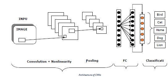
Creating CNN structure
We have seen the architecture and the basics of CNN, now we are going to building convolutional network using CNTK. Here, we will first see how to put together the structure of the CNN and then we will look at how to train the parameters of it.
At last we’ll see, how we can improve the neural network by changing its structure with various different layer setups. We are going to use MNIST image dataset.
So, first let’s create a CNN structure. Generally, when we build a CNN for recognizing patterns in images, we do the following−
We use a combination of convolution and pooling layers.
One or more hidden layer at the end of the network.
At last, we finish the network with a softmax layer for classification purpose.
With the help of following steps, we can build the network structure−
Step 1− First, we need to import the required layers for CNN.
from cntk.layers import Convolution2D, Sequential, Dense, MaxPooling
Step 2− Next, we need to import the activation functions for CNN.
from cntk.ops import log_softmax, relu
Step 3− After that in order to initialize the convolutional layers later, we need to import the glorot_uniform_initializer as follows−
from cntk.initializer import glorot_uniform
Step 4− Next, to create input variables import the input_variable function. And import default_option function, to make configuration of NN a bit easier.
from cntk import input_variable, default_options
Step 5− Now to store the input images, create a new input_variable. It will contain three channels namely red, green and blue. It would have the size of 28 by 28 pixels.
features = input_variable((3,28,28))
Step 6−Next, we need to create another input_variable to store the labels to predict.
labels = input_variable(10)
Step 7− Now, we need to create the default_option for the NN. And, we need to use the glorot_uniform as the initialization function.
with default_options(initialization=glorot_uniform, activation=relu):
Step 8− Next, in order to set the structure of the NN, we need to create a new Sequential layer set.
Step 9− Now we need to add a Convolutional2D layer with a filter_shape of 5 and a strides setting of 1, within the Sequential layer set. Also, enable padding, so that the image is padded to retain the original dimensions.
model = Sequential([
Convolution2D(filter_shape=(5,5), strides=(1,1), num_filters=8, pad=True),
Step 10− Now it’s time to add a MaxPooling layer with filter_shape of 2, and a strides setting of 2 to compress the image by half.
MaxPooling(filter_shape=(2,2), strides=(2,2)),
Step 11− Now, as we did in step 9, we need to add another Convolutional2D layer with a filter_shape of 5 and a strides setting of 1, use 16 filters. Also, enable padding, so that, the size of the image produced by the previous pooling layer should be retained.
Convolution2D(filter_shape=(5,5), strides=(1,1), num_filters=16, pad=True),
Step 12− Now, as we did in step 10, add another MaxPooling layer with a filter_shape of 3 and a strides setting of 3 to reduce the image to a third.
MaxPooling(filter_shape=(3,3), strides=(3,3)),
Step 13− At last, add a Dense layer with ten neurons for the 10 possible classes, the network can predict. In order to turn the network into a classification model, use a log_siftmax activation function.
Dense(10, activation=log_softmax)
])
Complete Example for creating CNN structure
from cntk.layers import Convolution2D, Sequential, Dense, MaxPooling
from cntk.ops import log_softmax, relu
from cntk.initializer import glorot_uniform
from cntk import input_variable, default_options
features = input_variable((3,28,28))
labels = input_variable(10)
with default_options(initialization=glorot_uniform, activation=relu):
model = Sequential([
   Convolution2D(filter_shape=(5,5), strides=(1,1), num_filters=8, pad=True),
MaxPooling(filter_shape=(2,2), strides=(2,2)),
   Convolution2D(filter_shape=(5,5), strides=(1,1), num_filters=16, pad=True),
MaxPooling(filter_shape=(3,3), strides=(3,3)),
Dense(10, activation=log_softmax)
])
z = model(features)
Training CNN with images
As we have created the structure of the network, it’s time to train the network. But before starting the training of our network, we need to set up minibatch sources, because training a NN that works with images requires more memory, than most computers have.
We have already created minibatch sources in previous sections. Following is the Python code to set up two minibatch sources −
As we have the create_datasource function, we can now create two separate data sources (training and testing one) to train the model.
train_datasource = create_datasource('mnist_train')
test_datasource = create_datasource('mnist_test', max_sweeps=1, train=False)
Now, as we have prepared the images, we can start training of our NN. As we did in previous sections, we can use the train method on the loss function to kick off the training. Following is the code for this −
from cntk import Function
from cntk.losses import cross_entropy_with_softmax
from cntk.metrics import classification_error
from cntk.learners import sgd
@Function
def criterion_factory(output, targets):
loss = cross_entropy_with_softmax(output, targets)
metric = classification_error(output, targets)
return loss, metric
loss = criterion_factory(z, labels)
learner = sgd(z.parameters, lr=0.2)
With the help of previous code, we have setup the loss and learner for the NN. The following code will train and validate the NN−
from cntk.logging import ProgressPrinter
from cntk.train import TestConfig
progress_writer = ProgressPrinter(0)
test_config = TestConfig(test_datasource)
input_map = {
   features: train_datasource.streams.features,
   labels: train_datasource.streams.labels
}
loss.train(train_datasource,
     max_epochs=10,
     minibatch_size=64,
     epoch_size=60000,
        parameter_learners=[learner],
     model_inputs_to_streams=input_map,
     callbacks=[progress_writer, test_config])
Complete Implementation Example
from cntk.layers import Convolution2D, Sequential, Dense, MaxPooling
from cntk.ops import log_softmax, relu
from cntk.initializer import glorot_uniform
from cntk import input_variable, default_options
features = input_variable((3,28,28))
labels = input_variable(10)
with default_options(initialization=glorot_uniform, activation=relu):
model = Sequential([
   Convolution2D(filter_shape=(5,5), strides=(1,1), num_filters=8, pad=True),
MaxPooling(filter_shape=(2,2), strides=(2,2)),
   Convolution2D(filter_shape=(5,5), strides=(1,1), num_filters=16, pad=True),
MaxPooling(filter_shape=(3,3), strides=(3,3)),
Dense(10, activation=log_softmax)
])
z = model(features)
import os
from cntk.io import MinibatchSource, StreamDef, StreamDefs, ImageDeserializer, INFINITELY_REPEAT
import cntk.io.transforms as xforms
def create_datasource(folder, train=True, max_sweeps=INFINITELY_REPEAT):
   mapping_file = os.path.join(folder, 'mapping.bin')
   image_transforms = []
   if train:
    image_transforms += [
     xforms.crop(crop_type='randomside', side_ratio=0.8),
     xforms.scale(width=28, height=28, channels=3, interpolations='linear')
]
   stream_definitions = StreamDefs(
   features=StreamDef(field='image', transforms=image_transforms),
    labels=StreamDef(field='label', shape=10)
)
   deserializer = ImageDeserializer(mapping_file, stream_definitions)
return MinibatchSource(deserializer, max_sweeps=max_sweeps)
train_datasource = create_datasource('mnist_train')
test_datasource = create_datasource('mnist_test', max_sweeps=1, train=False)
from cntk import Function
from cntk.losses import cross_entropy_with_softmax
from cntk.metrics import classification_error
from cntk.learners import sgd
@Function
def criterion_factory(output, targets):
   loss = cross_entropy_with_softmax(output, targets)
   metric = classification_error(output, targets)
return loss, metric
loss = criterion_factory(z, labels)
learner = sgd(z.parameters, lr=0.2)
from cntk.logging import ProgressPrinter
from cntk.train import TestConfig
progress_writer = ProgressPrinter(0)
test_config = TestConfig(test_datasource)
input_map = {
   features: train_datasource.streams.features,
   labels: train_datasource.streams.labels
}
loss.train(train_datasource,
     max_epochs=10,
     minibatch_size=64,
     epoch_size=60000,
        parameter_learners=[learner],
     model_inputs_to_streams=input_map,
     callbacks=[progress_writer, test_config])
Output
-------------------------------------------------------------------
average  since  average  since  examples
loss     last   metric   last
------------------------------------------------------
Learning rate per minibatch: 0.2
142      142      0.922   0.922    64
1.35e+06 1.51e+07 0.896   0.883    192
[………]
Image transformations
As we have seen, it’s difficult to train NN used for image recognition and, they require a lot of data to train also. One more issue is that, they tend to overfit on images used during training. Let us see with an example, when we have photos of faces in an upright position, our model will have a hard time recognizing faces that are rotated in another direction.
In order to overcome such problem, we can use image augmentation and CNTK supports specific transforms, when creating minibatch sources for images. We can use several transformations as follows−
We can randomly crop images used for training with just a few lines of code.
We can use a scale and color also.
Let’s see with the help of following Python code, how we can change the list of transformations by including a cropping transformation within the function used to create the minibatch source earlier.
import os
from cntk.io import MinibatchSource, StreamDef, StreamDefs, ImageDeserializer, INFINITELY_REPEAT
import cntk.io.transforms as xforms
def create_datasource(folder, train=True, max_sweeps=INFINITELY_REPEAT):
   mapping_file = os.path.join(folder, 'mapping.bin')
   image_transforms = []
   if train:
   image_transforms += [
     xforms.crop(crop_type='randomside', side_ratio=0.8),
xforms.scale(width=28, height=28, channels=3, interpolations='linear')
]
   stream_definitions = StreamDefs(
   features=StreamDef(field='image', transforms=image_transforms),
labels=StreamDef(field='label', shape=10)
)
   deserializer = ImageDeserializer(mapping_file, stream_definitions)
return MinibatchSource(deserializer, max_sweeps=max_sweeps)
With the help of above code, we can enhance the function to include a set of image transforms, so that, when we will be training we can randomly crop the image, so we get more variations of the image.
CNTK - Recurrent Neural Network
Now, let us understand how to construct a Recurrent Neural Network (RNN) in CNTK.
Introduction
We learned how to classify images with a neural network, and it is one of the iconic jobs in deep learning. But, another area where neural network excels at and lot of research happening is Recurrent Neural Networks (RNN). Here, we are going to know what RNN is and how it can be used in scenarios where we need to deal with time-series data.
What is Recurrent Neural Network?
Recurrent neural networks (RNNs) may be defined as the special breed of NNs that are capable of reasoning over time. RNNs are mainly used in scenarios, where we need to deal with values that change over time, i.e. time-series data. In order to understand it in a better way, let’s have a small comparison between regular neural networks and recurrent neural networks −
As we know that, in a regular neural network, we can provide only one input. This limits it to results in only one prediction. To give you an example, we can do translating text job by using regular neural networks.
On the other hand, in recurrent neural networks, we can provide a sequence of samples that result in a single prediction. In other words, using RNNs we can predict an output sequence based on an input sequence. For example, there have been quite a few successful experiments with RNN in translation tasks.
Uses of Recurrent Neural Network
RNNs can be used in several ways. Some of them are as follows −
Predicting a single output
Before getting deep dive into the steps, that how RNN can predict a single output based on a sequence, let’s see how a basic RNN looks like−
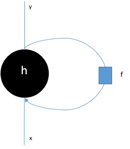
As we can in the above diagram, RNN contains a loopback connection to the input and whenever, we feed a sequence of values it will process each element in the sequence as time steps.
Moreover, because of the loopback connection, RNN can combine the generated output with input for the next element in the sequence. In this way, RNN will build a memory over the whole sequence which can be used to make a prediction.
In order to make prediction with RNN, we can perform the following steps−
First, to create an initial hidden state, we need to feed the first element of the input sequence.
After that, to produce an updated hidden state, we need to take the initial hidden state and combine it with the second element in the input sequence.
At last, to produce the final hidden state and to predict the output for the RNN, we need to take the final element in the input sequence.
In this way, with the help of this loopback connection we can teach a RNN to recognize patterns that happen over time.
Predicting a sequence
The basic model, discussed above, of RNN can be extended to other use cases as well. For example, we can use it to predict a sequence of values based on a single input. In this scenario, order to make prediction with RNN we can perform the following steps −
First, to create an initial hidden state and predict the first element in the output sequence, we need to feed an input sample into the neural network.
After that, to produce an updated hidden state and the second element in the output sequence, we need to combine the initial hidden state with the same sample.
At last, to update the hidden state one more time and predict the final element in output sequence, we feed the sample another time.
Predicting sequences
As we have seen how to predict a single value based on a sequence and how to predict a sequence based on a single value. Now let’s see how we can predict sequences for sequences. In this scenario, order to make prediction with RNN we can perform the following steps −
First, to create an initial hidden state and predict the first element in the output sequence, we need to take the first element in the input sequence.
After that, to update the hidden state and predict the second element in the output sequence, we need to take the initial hidden state.
At last, to predict the final element in the output sequence, we need to take the updated hidden state and the final element in the input sequence.
Working of RNN
To understand the working of recurrent neural networks (RNNs) we need to first understand how recurrent layers in the network work. So first let’s discuss how e can predict the output with a standard recurrent layer.
Predicting output with standard RNN layer
As we discussed earlier also that a basic layer in RNN is quite different from a regular layer in a neural network. In previous section, we also demonstrated in the diagram the basic architecture of RNN. In order to update the hidden state for the first-time step-in sequence we can use the following formula −
In the above equation, we calculate the new hidden state by calculating the dot product between the initial hidden state and a set of weights.
Now for the next step, the hidden state for the current time step is used as the initial hidden state for the next time step in the sequence. That’s why, to update the hidden state for the second time step, we can repeat the calculations performed in the first-time step as follows −
Next, we can repeat the process of updating the hidden state for the third and final step in the sequence as below −
And when we have processed all the above steps in the sequence, we can calculate the output as follows −
For the above formula, we have used a third set of weights and the hidden state from the final time step.
Advanced Recurrent Units
The main issue with basic recurrent layer is of vanishing gradient problem and due to this it is not very good at learning long-term correlations. In simple words basic recurrent layer does not handle long sequences very well. That’s the reason some other recurrent layer types that are much more suited for working with longer sequences are as follows −
Long-Short Term Memory (LSTM)

Long-short term memory (LSTMs) networks were introduced by Hochreiter & Schmidhuber. It solved the problem of getting a basic recurrent layer to remember things for a long time. The architecture of LSTM is given above in the diagram. As we can see it has input neurons, memory cells, and output neurons. In order to combat the vanishing gradient problem, Long-short term memory networks use an explicit memory cell (stores the previous values) and the following gates −
Forget gate− As name implies, it tells the memory cell to forget the previous values. The memory cell stores the values until the gate i.e. ‘forget gate’ tells it to forget them.
Input gate− As name implies, it adds new stuff to the cell.
Output gate− As name implies, output gate decides when to pass along the vectors from the cell to the next hidden state.
Gated Recurrent Units (GRUs)

Gradient recurrent units (GRUs) is a slight variation of LSTMs network. It has one less gate and are wired slightly different than LSTMs. Its architecture is shown in the above diagram. It has input neurons, gated memory cells, and output neurons. Gated Recurrent Units network has the following two gates −
Update gate− It determines the following two things−
What amount of the information should be kept from the last state?
What amount of the information should be let in from the previous layer?
Reset gate− The functionality of reset gate is much like that of forget gate of LSTMs network. The only difference is that it is located slightly differently.
In contrast to Long-short term memory network, Gated Recurrent Unit networks are slightly faster and easier to run.
Creating RNN structure
Before we can start, making prediction about the output from any of our data source, we need to first construct RNN and constructing RNN is quite same as we had build regular neural network in previous section. Following is the code to build one−
from cntk.losses import squared_error
from cntk.io import CTFDeserializer, MinibatchSource, INFINITELY_REPEAT, StreamDefs, StreamDef
from cntk.learners import adam
from cntk.logging import ProgressPrinter
from cntk.train import TestConfig
BATCH_SIZE = 14 * 10
EPOCH_SIZE = 12434
EPOCHS = 10
Staking multiple layers
We can also stack multiple recurrent layers in CNTK. For example, we can use the following combination of layers−
from cntk import sequence, default_options, input_variable
from cntk.layers import Recurrence, LSTM, Dropout, Dense, Sequential, Fold
features = sequence.input_variable(1)
with default_options(initial_state = 0.1):
   model = Sequential([
      Fold(LSTM(15)),
      Dense(1)
   ])(features)
target = input_variable(1, dynamic_axes=model.dynamic_axes)
As we can see in the above code, we have the following two ways in which we can model RNN in CNTK −
First, if we only want the final output of a recurrent layer, we can use the Fold layer in combination with a recurrent layer, such as GRU, LSTM, or even RNNStep.
Second, as an alternative way, we can also use the Recurrence block.
Training RNN with time series data
Once we build the model, let’s see how we can train RNN in CNTK −
from cntk import Function
@Function
def criterion_factory(z, t):
   loss = squared_error(z, t)
   metric = squared_error(z, t)
   return loss, metric
loss = criterion_factory(model, target)
learner = adam(model.parameters, lr=0.005, momentum=0.9)
Now to load the data into the training process, we must have to deserialize sequences from a set of CTF files. Following code have the create_datasource function, which is a useful utility function to create both the training and test datasource.
target_stream = StreamDef(field='target', shape=1, is_sparse=False)
features_stream = StreamDef(field='features', shape=1, is_sparse=False)
deserializer = CTFDeserializer(filename, StreamDefs(features=features_stream, target=target_stream))
   datasource = MinibatchSource(deserializer, randomize=True, max_sweeps=sweeps)
return datasource
train_datasource = create_datasource('Training data filename.ctf')#we need to provide the location of training file we created from our dataset.
test_datasource = create_datasource('Test filename.ctf', sweeps=1) #we need to provide the location of testing file we created from our dataset.
Now, as we have setup the data sources, model and the loss function, we can start the training process. It is quite similar as we did in previous sections with basic neural networks.
progress_writer = ProgressPrinter(0)
test_config = TestConfig(test_datasource)
input_map = {
   features: train_datasource.streams.features,
   target: train_datasource.streams.target
}
history = loss.train(
   train_datasource,
   epoch_size=EPOCH_SIZE,
   parameter_learners=[learner],
   model_inputs_to_streams=input_map,
   callbacks=[progress_writer, test_config],
   minibatch_size=BATCH_SIZE,
   max_epochs=EPOCHS
)
We will get the output similar as follows −
Output−
average  since  average  since  examples
loss      last  metric  last
------------------------------------------------------
Learning rate per minibatch: 0.005
0.4      0.4    0.4      0.4      19
0.4      0.4    0.4      0.4      59
0.452    0.495  0.452    0.495   129
[…]
Validating the model
Actually redicting with a RNN is quite similar to making predictions with any other CNK model. The only difference is that, we need to provide sequences rather than single samples.
Now, as our RNN is finally done with training, we can validate the model by testing it using a few samples sequence as follows −
import pickle
with open('test_samples.pkl', 'rb') as test_file:
test_samples = pickle.load(test_file)
model(test_samples) * NORMALIZE
Output−
array([[ 8081.7905],
[16597.693 ],
[13335.17 ],
...,
[11275.804 ],
[15621.697 ],
[16875.555 ]], dtype=float32)