- Matplotlib Tutorial
- Matplotlib - Home
- Matplotlib - Introduction
- Matplotlib - Environment Setup
- Matplotlib - Anaconda distribution
- Matplotlib - Jupyter Notebook
- Matplotlib - Pyplot API
- Matplotlib - Simple Plot
- Matplotlib - PyLab module
- Object-oriented Interface
- Matplotlib - Figure Class
- Matplotlib - Axes Class
- Matplotlib - Multiplots
- Matplotlib - Subplots() Function
- Matplotlib - Subplot2grid() Function
- Matplotlib - Grids
- Matplotlib - Formatting Axes
- Matplotlib - Setting Limits
- Setting Ticks and Tick Labels
- Matplotlib - Twin Axes
- Matplotlib - Bar Plot
- Matplotlib - Histogram
- Matplotlib - Pie Chart
- Matplotlib - Scatter Plot
- Matplotlib - Contour Plot
- Matplotlib - Quiver Plot
- Matplotlib - Box Plot
- Matplotlib - Violin Plot
- Three-dimensional Plotting
- Matplotlib - 3D Contour Plot
- Matplotlib - 3D Wireframe plot
- Matplotlib - 3D Surface plot
- Matplotlib - Working With Text
- Mathematical Expressions
- Matplotlib - Working with Images
- Matplotlib - Transforms
- Matplotlib Useful Resources
- Matplotlib - Quick Guide
- Matplotlib - Useful Resources
- Matplotlib - Discussion
Matplotlib - 3D Surface Plots
A 3D surface plot is a way to visualize data that has three dimensions: length, width, and height.
Imagine a landscape with hills and valleys where each point on the surface represents a specific value. In a 3D surface plot, these points are plotted in a three-dimensional space, creating a surface that shows how the data varies across different positions. It is like looking at a three-dimensional map of the data, where the height of the surface represents the value of the data at each point.
3D Surface Plot in Matplotlib
In Matplotlib, a 3D surface plot is a visual representation of multiple points connected like a graph with a specific area in three-dimensional space. We can create a 3d surface plot in Matplotlib using the plot_surface() function in "mpl_toolkits.mplot3d" module. It takes the X, Y, and Z coordinates as arrays and creates a continuous graph by joining the three coordinates.
Let’s start by drawing a basic 3D surface plot.
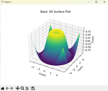
Basic 3D Surface Plot
A basic 3D surface plot in Matplotlib is way of representing a graph in three dimensions, with X, Y, and Z axes. The coordinates form a surface where height or depth (Z-axis) at each point gives the plot its three-dimensional shape.
Example
In the following example, we are creating a basic 3D surface plot by evenly spacing the X and Y coordinates and then finding the Z coordinate based on the values of X and Y coordinates −
import matplotlib.pyplot as plt
import numpy as np
from mpl_toolkits.mplot3d import Axes3D

# Creating data
x = np.linspace(-5, 5, 100)
y = np.linspace(-5, 5, 100)
X, Y = np.meshgrid(x, y)
Z = np.sin(np.sqrt(X**2 + Y**2))

# Creating a 3D plot
fig = plt.figure()
ax = fig.add_subplot(111, projection='3d')

# Plotting the basic 3D surface
ax.plot_surface(X, Y, Z, cmap='viridis')

# Customizing the plot
ax.set_xlabel('X-axis')
ax.set_ylabel('Y-axis')
ax.set_zlabel('Z-axis')
ax.set_title('Basic 3D Surface Plot')

# Displaying the plot
plt.show()
Output
Following is the output of the above code −
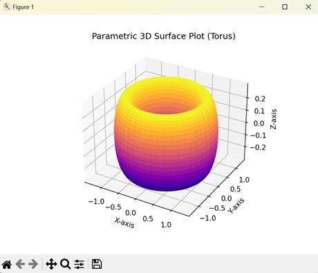
Parametric 3D Surface Plots
Parametric 3D surface plots in Matplotlib use mathematical equations to define a graph in three-dimensional space. These equations describe how the values of X, Y, and Z coordinates changes with variations in parameter values.
Example
In here, we are creating a parametric 3D surface plot by parametrizing the X, Y, and Z coordinates with respect to initial data points (u, v), size (R) and thickness (r). The resulting plot shows a donut-shaped surface plot −
import matplotlib.pyplot as plt
import numpy as np
from mpl_toolkits.mplot3d import Axes3D

# Parametric equations for a torus
def torus_parametric(u, v, R=1, r=0.3):
   x = (R + r * np.cos(v)) * np.cos(u)
   y = (R + r * np.cos(v)) * np.sin(u)
   z = r * np.sin(v)
   return x, y, z

# Generating data
u = np.linspace(0, 2 * np.pi, 100)
v = np.linspace(0, 2 * np.pi, 100)
U, V = np.meshgrid(u, v)
X, Y, Z = torus_parametric(U, V)

# Creating a 3D plot
fig = plt.figure()
ax = fig.add_subplot(111, projection='3d')

# Plotting the parametric 3D surface
ax.plot_surface(X, Y, Z, cmap='plasma')

# Customizing the plot
ax.set_xlabel('X-axis')
ax.set_ylabel('Y-axis')
ax.set_zlabel('Z-axis')
ax.set_title('Parametric 3D Surface Plot (Torus)')

# Displaying the plot
plt.show()
Output
On executing the above code we will get the following output −
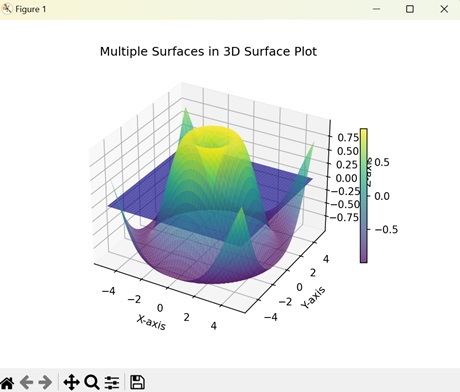
Multiple 3D Surface Plots
In Matplotlib, multiple 3D surface plots displays multiple graphs stacked on top of each other in a three-dimensional space. Each graph has a distinct value for the X, Y, and Z coordinates.
Example
The following example creates two 3D surface plots stacked on top of each other. We use different equations to create two distinct 3D surface plots. The resultant plot shows the two surface plots on different planes with different colors −
import matplotlib.pyplot as plt
import numpy as np
from mpl_toolkits.mplot3d import Axes3D

# Creating data for two surfaces
x = np.linspace(-5, 5, 100)
y = np.linspace(-5, 5, 100)
X, Y = np.meshgrid(x, y)
Z1 = np.sin(np.sqrt(X**2 + Y**2))
Z2 = np.exp(-(X**2 + Y**2))

# Creating a 3D plot
fig = plt.figure()
ax = fig.add_subplot(111, projection='3d')

# Plotting the two surfaces
surf1 = ax.plot_surface(X, Y, Z1, cmap='viridis', alpha=0.7)
surf2 = ax.plot_surface(X, Y, Z2, cmap='plasma', alpha=0.7)

# Customize the plot
ax.set_xlabel('X-axis')
ax.set_ylabel('Y-axis')
ax.set_zlabel('Z-axis')
ax.set_title('Multiple Surfaces in 3D Surface Plot')

# Adding a colorbar
fig.colorbar(surf1, ax=ax, orientation='vertical', shrink=0.5, aspect=20)

# Displaying the plot
plt.show()
Output
After executing the above code, we get the following output −
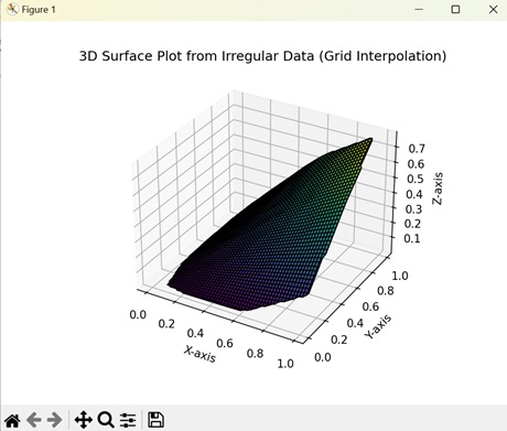
Interpolated 3D Surface Plots
Interpolated 3D surface plots in Matplotlib help us to visualize a graph whose X, Y, and Z coordinates are scattered randomly. Interpolation helps to fill in the missing data points to create a continuous graph.
Example
Now, we are creating an interpolated 3D surface plots. We generate random values for the X, Y, and Z coordinates and then use linear interpolation to estimate the values of missing data points using nearest data points −
import matplotlib.pyplot as plt
import numpy as np
from mpl_toolkits.mplot3d import Axes3D
from scipy.interpolate import griddata

# Creating irregularly spaced data
np.random.seed(42)
x = np.random.rand(100)
y = np.random.rand(100)
z = np.sin(x * y)

# Creating a regular grid
xi, yi = np.linspace(x.min(), x.max(), 100), np.linspace(y.min(), y.max(), 100)
xi, yi = np.meshgrid(xi, yi)

# Interpolating irregular data onto the regular grid
zi = griddata((x, y), z, (xi, yi), method='linear')

# Creating a 3D plot
fig = plt.figure()
ax = fig.add_subplot(111, projection='3d')

# Plotting the 3D surface from irregular data using grid interpolation
ax.plot_surface(xi, yi, zi, cmap='viridis', edgecolor='k')

# Customizing the plot
ax.set_xlabel('X-axis')
ax.set_ylabel('Y-axis')
ax.set_zlabel('Z-axis')
ax.set_title('3D Surface Plot from Irregular Data (Grid Interpolation)')

# Displaying the plot
plt.show()
Output
On executing the above code we will get the following output −