Regression Techniques

---

---

Regression is a statistical technique that helps in qualifying the relationship between the interrelated economic variables. The first step involves estimating the coefficient of the independent variable and then measuring the reliability of the estimated coefficient. This requires formulating a hypothesis, and based on the hypothesis, we can create a function.

If a manager wants to determine the relationship between the firm’s advertisement expenditures and its sales revenue, he will undergo the test of hypothesis. Assuming that higher advertising expenditures lead to higher sale for a firm. The manager collects data on advertising expenditure and on sales revenue in a specific period of time. This hypothesis can be translated into the mathematical function, where it leads to −

Y = A + Bx

Where Y is sales, x is the advertisement expenditure, A and B are constant.

After translating the hypothesis into the function, the basis for this is to find the relationship between the dependent and independent variables. The value of dependent variable is of most importance to researchers and depends on the value of other variables. Independent variable is used to explain the variation in the dependent variable. It can be classified into two types −

• Simple regression − One independent variable

• Multiple regression − Several independent variables

Simple Regression

Following are the steps to build up regression analysis −

• Specify the regression model
• Obtain data on variables
• Estimate the quantitative relationships
• Test the statistical significance of the results
• Usage of results in decision-making

Formula for simple regression is −

Y = a + bX + u

Y= dependent variable

X= independent variable

a= intercept

b= slope

u= random factor

Cross sectional data provides information on a group of entities at a given time, whereas time series data provides information on one entity over time. When we estimate regression equation it involves the process of finding out the best linear relationship between the dependent and the independent variables.

Method of Ordinary Least Squares (OLS)

Ordinary least square method is designed to fit a line through a scatter of points is such a way that the sum of the squared deviations of the points from the line is minimized. It is a statistical method. Usually Software packages perform OLS estimation.

Y = a + bX

Co-efficient of Determination (R²)

Co-efficient of determination is a measure which indicates the percentage of the variation in the dependent variable is due to the variations in the independent variables. R² is a measure of the goodness of fit model. Following are the methods −

Total Sum of Squares (TSS)

Sum of the squared deviations of the sample values of Y from the mean of Y.

TSS = SUM ( Y_i − Y)²

Y_i = dependent variables

Y = mean of dependent variables

i = number of observations

Regression Sum of Squares (RSS)

Sum of the squared deviations of the estimated values of Y from the mean of Y.

RSS = SUM ( Ỷ_i − uY)²

Ỷ_i = estimated value of Y

Y = mean of dependent variables

i = number of variations

Error Sum of Squares (ESS)

Sum of the squared deviations of the sample values of Y from the estimated values of Y.

ESS = SUM ( Y_i − Ỷ_i)²

Ỷ_i = estimated value of Y

Y_i = dependent variables

i = number of observations

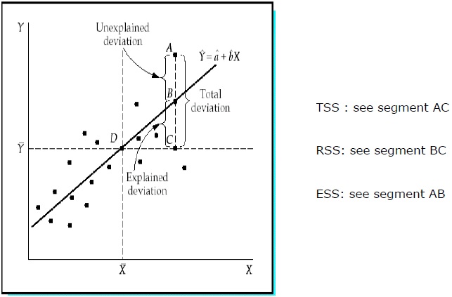
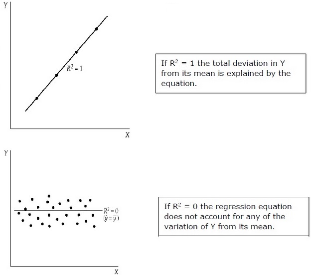
R² measures the proportion of the total deviation of Y from its mean which is explained by the regression model. The closer the R² is to unity, the greater the explanatory power of the regression equation. An R² close to 0 indicates that the regression equation will have very little explanatory power.

For evaluating the regression coefficients, a sample from the population is used rather than the entire population. It is important to make assumptions about the population based on the sample and to make a judgment about how good these assumptions are.

Evaluating the Regression Coefficients

Each sample from the population generates its own intercept. To calculate the statistical difference following methods can be used −

Two tailed test −

Null Hypothesis: H₀: b = 0

Alternative Hypothesis: H_a: b ≠ 0

One tailed test −

Null Hypothesis: H₀: b > 0 (or b < 0)

Alternative Hypothesis: H_a: b < 0 (or b > 0)

Statistic Test −

b = estimated coefficient

E (b) = b = 0 (Null hypothesis)

SE_b = Standard error of the coefficient

.

Value of t depends on the degree of freedom, one or two failed test, and level of significance. To determine the critical value of t, t-table can be used. Then comes the comparison of the t-value with the critical value. One needs to reject the null hypothesis if the absolute value of the statistic test is greater than or equal to the critical t-value. Do not reject the null hypothesis, I the absolute value of the statistic test is less than the critical t–value.

Multiple Regression Analysis

Unlike simple regression in multiple regression analysis, the coefficients indicate the change in dependent variables assuming the values of the other variables are constant.

The test of statistical significance is called F-test. The F-test is useful as it measures the statistical significance of the entire regression equation rather than just for an individual. Here In null hypothesis, there is no relationship between the dependent variable and the independent variables of the population.

The formula is − H₀: b1 = b2 = b3 = …. = bk = 0

No relationship exists between the dependent variable and the k independent variables for the population.

F-test static −

$$F \: =\: \frac{ \left ( \frac{R^2}{K} \right )}{\frac{(1-R^2)}{(n-k-1)}}$$

Critical value of F depends on the numerator and denominator degree of freedom and level of significance. F-table can be used to determine the critical F–value. In comparison to F–value with the critical value (F*) −

If F > F*, we need to reject the null hypothesis.

If F < F*, do not reject the null hypothesis as there is no significant relationship between the dependent variable and all independent variables.