Machine Learning - Logistic Regression

---

---

Logistic regression is a popular algorithm used for binary classification problems, where the target variable is categorical with two classes. It models the probability of the target variable given the input features and predicts the class with the highest probability.

Logistic regression is a type of generalized linear model, where the target variable follows a Bernoulli distribution. The model consists of a linear function of the input features, which is transformed using the logistic function to produce a probability value between 0 and 1.

The linear function is basically used as an input to another function such as g in the following relation −

$$h_{\theta }\left ( x \right )=g\left ( \theta ^{T}x \right )\, where\: 0\leq h_{\theta }\leq 1$$

Here, g is the logistic or sigmoid function which can be given as follows −

$$g\left ( z \right )=\frac{1}{1+e^{-z}}\: where\: z=\theta ^{T}x$$

The sigmoid curve can be represented with the help of following graph. We can see the values of y-axis lie between 0 and 1 and crosses the axis at 0.5.

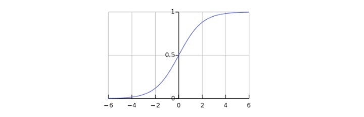
The classes can be divided into positive or negative. The output comes under the probability of positive class if it lies between 0 and 1. For our implementation, we are interpreting the output of hypothesis function as positive if it is ≥ 0.5, otherwise negative.

Implementation in Python

Now we will implement the above concept of logistic regression in Python. For this purpose, we are using a multivariate flower dataset named 'iris'. The iris dataset is a well-known dataset in machine learning, consisting of measurements of the sepal length, sepal width, petal length, and petal width of three different species of iris flowers. We will use logistic regression to predict the species of an iris flower given its measurements.

Let us now check the steps to implement logistic regression in Python using the iris dataset −

Load the Dataset

First, we need to load the iris dataset into our Python environment. We can use the scikitlearn library to load the dataset, as follows −

from sklearn.datasets import load_iris
iris = load_iris()
X = iris.data # input features
y = iris.target # target variable

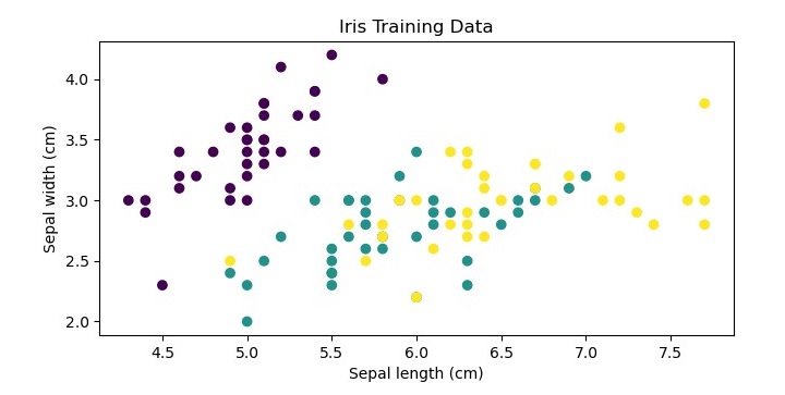
Plot the Training Data

This is an optional step but for more clarification about the dataset we are plotting the training data as follows −

import matplotlib.pyplot as plt

# plot the training data
plt.scatter(X_train[:, 0], X_train[:, 1], c=y_train)
plt.xlabel('Sepal length (cm)')
plt.ylabel('Sepal width (cm)')
plt.title('Iris Training Data')
plt.show()

Split the Dataset

Next, we need to split the dataset into a training set and a test set. We will use 70% of the data for training and 30% for testing.

from sklearn.model_selection import train_test_split

X_train, X_test, y_train, y_test = train_test_split(X, y, test_size=0.3,
random_state=42)

Create the Logistic Regression Model

We can use the LogisticRegression class from scikit-learn to create a logistic regression model. We will use L2 regularization and set the regularization strength to 1.

from sklearn.linear_model import LogisticRegression
clf = LogisticRegression(penalty='l2', C=1.0, random_state=42)

Train the Model

We can train the model on the training set using the fit() method.

clf.fit(X_train, y_train)

Make Predictions

Once the model is trained, we can use it to make predictions on the test set using the predict() method.

y_pred = clf.predict(X_test)

Evaluate the Model

Finally, we can evaluate the performance of the model using metrics such as accuracy, precision, recall, and F1-score.

from sklearn.metrics import accuracy_score, precision_score,
recall_score, f1_score
print('Accuracy:', accuracy_score(y_test, y_pred))
print('Precision:', precision_score(y_test, y_pred, average='macro'))
print('Recall:', recall_score(y_test, y_pred, average='macro'))
print('F1-score:', f1_score(y_test, y_pred, average='macro'))

Here, we have used the average parameter with the value 'macro' to calculate the metrics for each class separately and then take the average.

Complete Implementation Example

Give below is the complete implementation example of logistic regression in python using the iris dataset −

from sklearn.datasets import load_iris
from sklearn.model_selection import train_test_split
from sklearn.linear_model import LogisticRegression
import matplotlib.pyplot as plt
from sklearn.metrics import accuracy_score, precision_score, recall_score, f1_score

# load the iris dataset
iris = load_iris()
X = iris.data # input features
y = iris.target # target variable

# plot the training data
plt.figure(figsize=(7.5, 3.5))
plt.scatter(X_train[:, 0], X_train[:, 1], c=y_train)
plt.xlabel('Sepal length (cm)')
plt.ylabel('Sepal width (cm)')
plt.title('Iris Training Data')
plt.show()

# split the dataset into training and test sets
X_train, X_test, y_train, y_test = train_test_split(X, y, test_size=0.3, random_state=42)

# create the logistic regression model
clf = LogisticRegression(penalty='l2', C=1.0, random_state=42)

# train the model on the training set
clf.fit(X_train, y_train)

# make predictions on the test set
y_pred = clf.predict(X_test)

# evaluate the performance of the model
print('Accuracy:', accuracy_score(y_test, y_pred))
print('Precision:', precision_score(y_test, y_pred, average='macro'))
print('Recall:', recall_score(y_test, y_pred, average='macro'))
print('F1-score:', f1_score(y_test, y_pred, average='macro'))

Output

When you execute this code, it will produce the following plot as the output −

Accuracy: 1.0
Precision: 1.0
Recall: 1.0
F1-score: 1.0