- Logistic Regression in Python Tutorial
- Home
- Introduction
- Case Study
- Setting up a Project
- Getting Data
- Restructuring Data
- Preparing Data
- Splitting Data
- Building Classifier
- Testing
- Limitations
- Summary
- Logistic Regression in Python Resources
- Quick Guide
- Useful Resources
- Discussion
Logistic Regression in Python - Quick Guide
Logistic Regression in Python - Introduction
Logistic Regression is a statistical method of classification of objects. This chapter will give an introduction to logistic regression with the help of some examples.
Classification
To understand logistic regression, you should know what classification means. Let us consider the following examples to understand this better −
- A doctor classifies the tumor as malignant or benign.
- A bank transaction may be fraudulent or genuine.
For many years, humans have been performing such tasks - albeit they are error-prone. The question is can we train machines to do these tasks for us with a better accuracy?
One such example of machine doing the classification is the email Client on your machine that classifies every incoming mail as “spam” or “not spam” and it does it with a fairly large accuracy. The statistical technique of logistic regression has been successfully applied in email client. In this case, we have trained our machine to solve a classification problem.
Logistic Regression is just one part of machine learning used for solving this kind of binary classification problem. There are several other machine learning techniques that are already developed and are in practice for solving other kinds of problems.
If you have noted, in all the above examples, the outcome of the predication has only two values - Yes or No. We call these as classes - so as to say we say that our classifier classifies the objects in two classes. In technical terms, we can say that the outcome or target variable is dichotomous in nature.
There are other classification problems in which the output may be classified into more than two classes. For example, given a basket full of fruits, you are asked to separate fruits of different kinds. Now, the basket may contain Oranges, Apples, Mangoes, and so on. So when you separate out the fruits, you separate them out in more than two classes. This is a multivariate classification problem.
Logistic Regression in Python - Case Study
Consider that a bank approaches you to develop a machine learning application that will help them in identifying the potential clients who would open a Term Deposit (also called Fixed Deposit by some banks) with them. The bank regularly conducts a survey by means of telephonic calls or web forms to collect information about the potential clients. The survey is general in nature and is conducted over a very large audience out of which many may not be interested in dealing with this bank itself. Out of the rest, only a few may be interested in opening a Term Deposit. Others may be interested in other facilities offered by the bank. So the survey is not necessarily conducted for identifying the customers opening TDs. Your task is to identify all those customers with high probability of opening TD from the humongous survey data that the bank is going to share with you.
Fortunately, one such kind of data is publicly available for those aspiring to develop machine learning models. This data was prepared by some students at UC Irvine with external funding. The database is available as a part of UCI Machine Learning Repository and is widely used by students, educators, and researchers all over the world. The data can be downloaded from here.
In the next chapters, let us now perform the application development using the same data.
Setting Up a Project
In this chapter, we will understand the process involved in setting up a project to perform logistic regression in Python, in detail.
Installing Jupyter
We will be using Jupyter - one of the most widely used platforms for machine learning. If you do not have Jupyter installed on your machine, download it from here. For installation, you can follow the instructions on their site to install the platform. As the site suggests, you may prefer to use Anaconda Distribution which comes along with Python and many commonly used Python packages for scientific computing and data science. This will alleviate the need for installing these packages individually.
After the successful installation of Jupyter, start a new project, your screen at this stage would look like the following ready to accept your code.
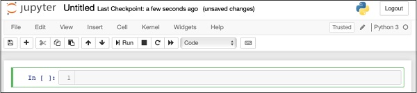
Now, change the name of the project from Untitled1 to “Logistic Regression” by clicking the title name and editing it.
First, we will be importing several Python packages that we will need in our code.
Importing Python Packages
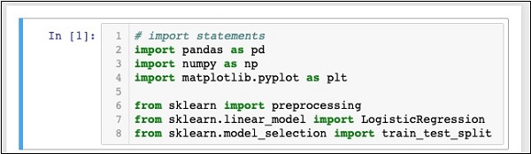
For this purpose, type or cut-and-paste the following code in the code editor −
In [1]: # import statements
   import pandas as pd
   import numpy as np
   import matplotlib.pyplot as plt

   from sklearn import preprocessing
   from sklearn.linear_model import LogisticRegression
   from sklearn.model_selection import train_test_split
Your Notebook should look like the following at this stage −
Run the code by clicking on the Run button. If no errors are generated, you have successfully installed Jupyter and are now ready for the rest of the development.
The first three import statements import pandas, numpy and matplotlib.pyplot packages in our project. The next three statements import the specified modules from sklearn.
Our next task is to download the data required for our project. We will learn this in the next chapter.
Logistic Regression in Python - Getting Data
The steps involved in getting data for performing logistic regression in Python are discussed in detail in this chapter.
Downloading Dataset
If you have not already downloaded the UCI dataset mentioned earlier, download it now from here. Click on the Data Folder. You will see the following screen −
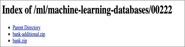
Download the bank.zip file by clicking on the given link. The zip file contains the following files −
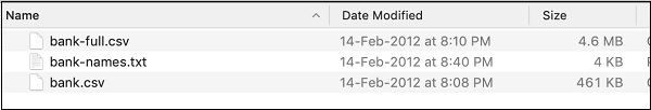
We will use the bank.csv file for our model development. The bank-names.txt file contains the description of the database that you are going to need later. The bank-full.csv contains a much larger dataset that you may use for more advanced developments.
Here we have included the bank.csv file in the downloadable source zip. This file contains the comma-delimited fields. We have also made a few modifications in the file. It is recommended that you use the file included in the project source zip for your learning.
Loading Data
To load the data from the csv file that you copied just now, type the following statement and run the code.
In [2]: df = pd.read_csv('bank.csv', header=0)
You will also be able to examine the loaded data by running the following code statement −
IN [3]: df.head()
Once the command is run, you will see the following output −
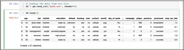
Basically, it has printed the first five rows of the loaded data. Examine the 21 columns present. We will be using only few columns from these for our model development.
Next, we need to clean the data. The data may contain some rows with NaN. To eliminate such rows, use the following command −
IN [4]: df = df.dropna()
Fortunately, the bank.csv does not contain any rows with NaN, so this step is not truly required in our case. However, in general it is difficult to discover such rows in a huge database. So it is always safer to run the above statement to clean the data.
Note − You can easily examine the data size at any point of time by using the following statement −
IN [5]: print (df.shape)
(41188, 21)
The number of rows and columns would be printed in the output as shown in the second line above.
Next thing to do is to examine the suitability of each column for the model that we are trying to build.
Logistic Regression in Python - Restructuring Data
Whenever any organization conducts a survey, they try to collect as much information as possible from the customer, with the idea that this information would be useful to the organization one way or the other, at a later point of time. To solve the current problem, we have to pick up the information that is directly relevant to our problem.
Displaying All Fields
Now, let us see how to select the data fields useful to us. Run the following statement in the code editor.
In [6]: print(list(df.columns))
You will see the following output −
['age', 'job', 'marital', 'education', 'default', 'housing', 'loan',
'contact', 'month', 'day_of_week', 'duration', 'campaign', 'pdays',
'previous', 'poutcome', 'emp_var_rate', 'cons_price_idx', 'cons_conf_idx',
'euribor3m', 'nr_employed', 'y']
The output shows the names of all the columns in the database. The last column “y” is a Boolean value indicating whether this customer has a term deposit with the bank. The values of this field are either “y” or “n”. You can read the description and purpose of each column in the banks-name.txt file that was downloaded as part of the data.
Eliminating Unwanted Fields
Examining the column names, you will know that some of the fields have no significance to the problem at hand. For example, fields such as month, day_of_week, campaign, etc. are of no use to us. We will eliminate these fields from our database. To drop a column, we use the drop command as shown below −
In [8]: #drop columns which are not needed.
   df.drop(df.columns[[0, 3, 7, 8, 9, 10, 11, 12, 13, 15, 16, 17, 18, 19]],
   axis = 1, inplace = True)
The command says that drop column number 0, 3, 7, 8, and so on. To ensure that the index is properly selected, use the following statement −
In [7]: df.columns[9]
Out[7]: 'day_of_week'
This prints the column name for the given index.
After dropping the columns which are not required, examine the data with the head statement. The screen output is shown here −
In [9]: df.head()
Out[9]:
      job   marital  default  housing  loan  poutcome    y
0     blue-collar    married  unknown yes no nonexistent 0
1     technician     married  no    no    no nonexistent 0
2     management     single   no    yes   no success     1
3     services       married  no    no    no nonexistent 0
4     retired        married  no    yes   no success     1
Now, we have only the fields which we feel are important for our data analysis and prediction. The importance of Data Scientist comes into picture at this step. The data scientist has to select the appropriate columns for model building.
For example, the type of job though at the first glance may not convince everybody for inclusion in the database, it will be a very useful field. Not all types of customers will open the TD. The lower income people may not open the TDs, while the higher income people will usually park their excess money in TDs. So the type of job becomes significantly relevant in this scenario. Likewise, carefully select the columns which you feel will be relevant for your analysis.
In the next chapter, we will prepare our data for building the model.
Logistic Regression in Python - Preparing Data
For creating the classifier, we must prepare the data in a format that is asked by the classifier building module. We prepare the data by doing One Hot Encoding.
Encoding Data
We will discuss shortly what we mean by encoding data. First, let us run the code. Run the following command in the code window.
In [10]: # creating one hot encoding of the categorical columns.
data = pd.get_dummies(df, columns =['job', 'marital', 'default', 'housing', 'loan', 'poutcome'])
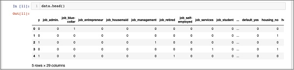
As the comment says, the above statement will create the one hot encoding of the data. Let us see what has it created? Examine the created data called “data” by printing the head records in the database.
In [11]: data.head()
You will see the following output −
To understand the above data, we will list out the column names by running the data.columns command as shown below −
In [12]: data.columns
Out[12]: Index(['y', 'job_admin.', 'job_blue-collar', 'job_entrepreneur',
'job_housemaid', 'job_management', 'job_retired', 'job_self-employed',
'job_services', 'job_student', 'job_technician', 'job_unemployed',
'job_unknown', 'marital_divorced', 'marital_married', 'marital_single',
'marital_unknown', 'default_no', 'default_unknown', 'default_yes',
'housing_no', 'housing_unknown', 'housing_yes', 'loan_no',
'loan_unknown', 'loan_yes', 'poutcome_failure', 'poutcome_nonexistent',
'poutcome_success'], dtype='object')
Now, we will explain how the one hot encoding is done by the get_dummies command. The first column in the newly generated database is “y” field which indicates whether this client has subscribed to a TD or not. Now, let us look at the columns which are encoded. The first encoded column is “job”. In the database, you will find that the “job” column has many possible values such as “admin”, “blue-collar”, “entrepreneur”, and so on. For each possible value, we have a new column created in the database, with the column name appended as a prefix.
Thus, we have columns called “job_admin”, “job_blue-collar”, and so on. For each encoded field in our original database, you will find a list of columns added in the created database with all possible values that the column takes in the original database. Carefully examine the list of columns to understand how the data is mapped to a new database.
Understanding Data Mapping
To understand the generated data, let us print out the entire data using the data command. The partial output after running the command is shown below.
In [13]: data
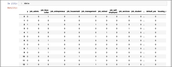
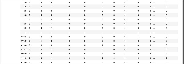
The above screen shows the first twelve rows. If you scroll down further, you would see that the mapping is done for all the rows.
A partial screen output further down the database is shown here for your quick reference.
To understand the mapped data, let us examine the first row.

It says that this customer has not subscribed to TD as indicated by the value in the “y” field. It also indicates that this customer is a “blue-collar” customer. Scrolling down horizontally, it will tell you that he has a “housing” and has taken no “loan”.
After this one hot encoding, we need some more data processing before we can start building our model.
Dropping the “unknown”
If we examine the columns in the mapped database, you will find the presence of few columns ending with “unknown”. For example, examine the column at index 12 with the following command shown in the screenshot −
In [14]: data.columns[12]
Out[14]: 'job_unknown'
This indicates the job for the specified customer is unknown. Obviously, there is no point in including such columns in our analysis and model building. Thus, all columns with the “unknown” value should be dropped. This is done with the following command −
In [15]: data.drop(data.columns[[12, 16, 18, 21, 24]], axis=1, inplace=True)
Ensure that you specify the correct column numbers. In case of a doubt, you can examine the column name anytime by specifying its index in the columns command as described earlier.
After dropping the undesired columns, you can examine the final list of columns as shown in the output below −
In [16]: data.columns
Out[16]: Index(['y', 'job_admin.', 'job_blue-collar', 'job_entrepreneur',
'job_housemaid', 'job_management', 'job_retired', 'job_self-employed',
'job_services', 'job_student', 'job_technician', 'job_unemployed',
'marital_divorced', 'marital_married', 'marital_single', 'default_no',
'default_yes', 'housing_no', 'housing_yes', 'loan_no', 'loan_yes',
'poutcome_failure', 'poutcome_nonexistent', 'poutcome_success'],
dtype='object')
At this point, our data is ready for model building.
Logistic Regression in Python - Splitting Data
We have about forty-one thousand and odd records. If we use the entire data for model building, we will not be left with any data for testing. So generally, we split the entire data set into two parts, say 70/30 percentage. We use 70% of the data for model building and the rest for testing the accuracy in prediction of our created model. You may use a different splitting ratio as per your requirement.
Creating Features Array
Before we split the data, we separate out the data into two arrays X and Y. The X array contains all the features (data columns) that we want to analyze and Y array is a single dimensional array of boolean values that is the output of the prediction. To understand this, let us run some code.
Firstly, execute the following Python statement to create the X array −
In [17]: X = data.iloc[:,1:]
To examine the contents of X use head to print a few initial records. The following screen shows the contents of the X array.
In [18]: X.head ()
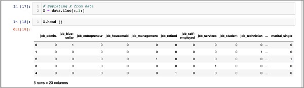
The array has several rows and 23 columns.
Next, we will create output array containing “y” values.
Creating Output Array
To create an array for the predicted value column, use the following Python statement −
In [19]: Y = data.iloc[:,0]
Examine its contents by calling head. The screen output below shows the result −
In [20]: Y.head()
Out[20]: 0   0
1    0
2    1
3    0
4    1
Name: y, dtype: int64
Now, split the data using the following command −
In [21]: X_train, X_test, Y_train, Y_test = train_test_split(X, Y, random_state=0)
This will create the four arrays called X_train, Y_train, X_test, and Y_test. As before, you may examine the contents of these arrays by using the head command. We will use X_train and Y_train arrays for training our model and X_test and Y_test arrays for testing and validating.
Now, we are ready to build our classifier. We will look into it in the next chapter.
Logistic Regression in Python - Building Classifier
It is not required that you have to build the classifier from scratch. Building classifiers is complex and requires knowledge of several areas such as Statistics, probability theories, optimization techniques, and so on. There are several pre-built libraries available in the market which have a fully-tested and very efficient implementation of these classifiers. We will use one such pre-built model from the sklearn.
The sklearn Classifier
Creating the Logistic Regression classifier from sklearn toolkit is trivial and is done in a single program statement as shown here −
In [22]: classifier = LogisticRegression(solver='lbfgs',random_state=0)
Once the classifier is created, you will feed your training data into the classifier so that it can tune its internal parameters and be ready for the predictions on your future data. To tune the classifier, we run the following statement −
In [23]: classifier.fit(X_train, Y_train)
The classifier is now ready for testing. The following code is the output of execution of the above two statements −
Out[23]: LogisticRegression(C = 1.0, class_weight = None, dual = False,
   fit_intercept=True, intercept_scaling=1, max_iter=100,
   multi_class='warn', n_jobs=None, penalty='l2', random_state=0,
   solver='lbfgs', tol=0.0001, verbose=0, warm_start=False))
Now, we are ready to test the created classifier. We will deal this in the next chapter.
Logistic Regression in Python - Testing
We need to test the above created classifier before we put it into production use. If the testing reveals that the model does not meet the desired accuracy, we will have to go back in the above process, select another set of features (data fields), build the model again, and test it. This will be an iterative step until the classifier meets your requirement of desired accuracy. So let us test our classifier.
Predicting Test Data
To test the classifier, we use the test data generated in the earlier stage. We call the predict method on the created object and pass the X array of the test data as shown in the following command −
In [24]: predicted_y = classifier.predict(X_test)
This generates a single dimensional array for the entire training data set giving the prediction for each row in the X array. You can examine this array by using the following command −
In [25]: predicted_y
The following is the output upon the execution the above two commands −
Out[25]: array([0, 0, 0, ..., 0, 0, 0])
The output indicates that the first and last three customers are not the potential candidates for the Term Deposit. You can examine the entire array to sort out the potential customers. To do so, use the following Python code snippet −
In [26]: for x in range(len(predicted_y)):
   if (predicted_y[x] == 1):
      print(x, end="\t")
The output of running the above code is shown below −
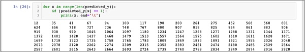
The output shows the indexes of all rows who are probable candidates for subscribing to TD. You can now give this output to the bank’s marketing team who would pick up the contact details for each customer in the selected row and proceed with their job.
Before we put this model into production, we need to verify the accuracy of prediction.
Verifying Accuracy
To test the accuracy of the model, use the score method on the classifier as shown below −
In [27]: print('Accuracy: {:.2f}'.format(classifier.score(X_test, Y_test)))
The screen output of running this command is shown below −
Accuracy: 0.90
It shows that the accuracy of our model is 90% which is considered very good in most of the applications. Thus, no further tuning is required. Now, our customer is ready to run the next campaign, get the list of potential customers and chase them for opening the TD with a probable high rate of success.
Logistic Regression in Python - Limitations
As you have seen from the above example, applying logistic regression for machine learning is not a difficult task. However, it comes with its own limitations. The logistic regression will not be able to handle a large number of categorical features. In the example we have discussed so far, we reduced the number of features to a very large extent.
However, if these features were important in our prediction, we would have been forced to include them, but then the logistic regression would fail to give us a good accuracy. Logistic regression is also vulnerable to overfitting. It cannot be applied to a non-linear problem. It will perform poorly with independent variables which are not correlated to the target and are correlated to each other. Thus, you will have to carefully evaluate the suitability of logistic regression to the problem that you are trying to solve.
There are many areas of machine learning where other techniques are specified devised. To name a few, we have algorithms such as k-nearest neighbours (kNN), Linear Regression, Support Vector Machines (SVM), Decision Trees, Naive Bayes, and so on. Before finalizing on a particular model, you will have to evaluate the applicability of these various techniques to the problem that we are trying to solve.
Logistic Regression in Python - Summary
Logistic Regression is a statistical technique of binary classification. In this tutorial, you learned how to train the machine to use logistic regression. Creating machine learning models, the most important requirement is the availability of the data. Without adequate and relevant data, you cannot simply make the machine to learn.
Once you have data, your next major task is cleansing the data, eliminating the unwanted rows, fields, and select the appropriate fields for your model development. After this is done, you need to map the data into a format required by the classifier for its training. Thus, the data preparation is a major task in any machine learning application. Once you are ready with the data, you can select a particular type of classifier.
In this tutorial, you learned how to use a logistic regression classifier provided in the sklearn library. To train the classifier, we use about 70% of the data for training the model. We use the rest of the data for testing. We test the accuracy of the model. If this is not within acceptable limits, we go back to selecting the new set of features.
Once again, follow the entire process of preparing data, train the model, and test it, until you are satisfied with its accuracy. Before taking up any machine learning project, you must learn and have exposure to a wide variety of techniques which have been developed so far and which have been applied successfully in the industry.