- Logistic Regression in Python Tutorial
- Home
- Introduction
- Case Study
- Setting up a Project
- Getting Data
- Restructuring Data
- Preparing Data
- Splitting Data
- Building Classifier
- Testing
- Limitations
- Summary
- Logistic Regression in Python Resources
- Quick Guide
- Useful Resources
- Discussion
Logistic Regression in Python - Preparing Data
For creating the classifier, we must prepare the data in a format that is asked by the classifier building module. We prepare the data by doing One Hot Encoding.
Encoding Data
We will discuss shortly what we mean by encoding data. First, let us run the code. Run the following command in the code window.
In [10]: # creating one hot encoding of the categorical columns.
data = pd.get_dummies(df, columns =['job', 'marital', 'default', 'housing', 'loan', 'poutcome'])
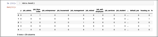
As the comment says, the above statement will create the one hot encoding of the data. Let us see what has it created? Examine the created data called “data” by printing the head records in the database.
In [11]: data.head()
You will see the following output −
To understand the above data, we will list out the column names by running the data.columns command as shown below −
In [12]: data.columns
Out[12]: Index(['y', 'job_admin.', 'job_blue-collar', 'job_entrepreneur',
'job_housemaid', 'job_management', 'job_retired', 'job_self-employed',
'job_services', 'job_student', 'job_technician', 'job_unemployed',
'job_unknown', 'marital_divorced', 'marital_married', 'marital_single',
'marital_unknown', 'default_no', 'default_unknown', 'default_yes',
'housing_no', 'housing_unknown', 'housing_yes', 'loan_no',
'loan_unknown', 'loan_yes', 'poutcome_failure', 'poutcome_nonexistent',
'poutcome_success'], dtype='object')
Now, we will explain how the one hot encoding is done by the get_dummies command. The first column in the newly generated database is “y” field which indicates whether this client has subscribed to a TD or not. Now, let us look at the columns which are encoded. The first encoded column is “job”. In the database, you will find that the “job” column has many possible values such as “admin”, “blue-collar”, “entrepreneur”, and so on. For each possible value, we have a new column created in the database, with the column name appended as a prefix.
Thus, we have columns called “job_admin”, “job_blue-collar”, and so on. For each encoded field in our original database, you will find a list of columns added in the created database with all possible values that the column takes in the original database. Carefully examine the list of columns to understand how the data is mapped to a new database.
Understanding Data Mapping
To understand the generated data, let us print out the entire data using the data command. The partial output after running the command is shown below.
In [13]: data
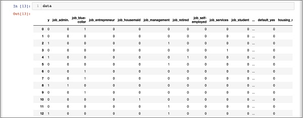
The above screen shows the first twelve rows. If you scroll down further, you would see that the mapping is done for all the rows.
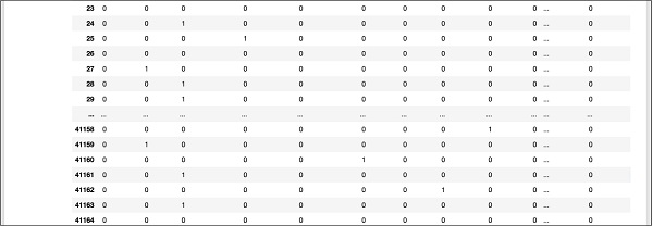
A partial screen output further down the database is shown here for your quick reference.
To understand the mapped data, let us examine the first row.

It says that this customer has not subscribed to TD as indicated by the value in the “y” field. It also indicates that this customer is a “blue-collar” customer. Scrolling down horizontally, it will tell you that he has a “housing” and has taken no “loan”.
After this one hot encoding, we need some more data processing before we can start building our model.
Dropping the “unknown”
If we examine the columns in the mapped database, you will find the presence of few columns ending with “unknown”. For example, examine the column at index 12 with the following command shown in the screenshot −
In [14]: data.columns[12]
Out[14]: 'job_unknown'
This indicates the job for the specified customer is unknown. Obviously, there is no point in including such columns in our analysis and model building. Thus, all columns with the “unknown” value should be dropped. This is done with the following command −
In [15]: data.drop(data.columns[[12, 16, 18, 21, 24]], axis=1, inplace=True)
Ensure that you specify the correct column numbers. In case of a doubt, you can examine the column name anytime by specifying its index in the columns command as described earlier.
After dropping the undesired columns, you can examine the final list of columns as shown in the output below −
In [16]: data.columns
Out[16]: Index(['y', 'job_admin.', 'job_blue-collar', 'job_entrepreneur',
'job_housemaid', 'job_management', 'job_retired', 'job_self-employed',
'job_services', 'job_student', 'job_technician', 'job_unemployed',
'marital_divorced', 'marital_married', 'marital_single', 'default_no',
'default_yes', 'housing_no', 'housing_yes', 'loan_no', 'loan_yes',
'poutcome_failure', 'poutcome_nonexistent', 'poutcome_success'],
dtype='object')
At this point, our data is ready for model building.