- KDB+ Tutorial
- KDB+ - Home
- KDB+ Architecture
- KDB+ - Overview
- KDB+ - Architecture
- Q Programming Language
- Q Programming Language
- Q Language - Type Casting
- Q Language - Temporal Data
- Q Language - Lists
- Q Language - Indexing
- Q Language - Dictionaries
- Q Language - Table
- Q Language - Verb & Adverbs
- Q Language - Joins
- Q Language - Functions
- Q Language - Built-in Functions
- Q Language - Queries
- Q - Inter-Process Communication
- Q - Message Handler (.Z Library)
- Q Advanced Topics
- Q Language - Attributes
- Q Language - Functional Queries
- Q Language - Table Arithmetic
- Q Language - Tables on Disk
- Q Language - Maintenance Functions
- KDB+ Useful Resources
- KDB+ - Quick Guide
- KDB+ - Useful Resources
- KDB+ - Discussion
KDB+ - Quick Guide
KDB+ - Overview
This is a complete quide to kdb+ from kx systems, aimed primarily at those learning independently. kdb+, introduced in 2003, is the new generation of the kdb database which is designed to capture, analyze, compare, and store data.
A kdb+ system contains the following two components −
KDB+ − the database (k database plus)
Q − the programming language for working with kdb+
Both kdb+ and q are written in k programming language (same as q but less readable).
Background
Kdb+/q originated as an obscure academic language but over the years, it has gradually improved its user friendliness.
APL (1964, A Programming Language)
A+ (1988, modified APL by Arthur Whitney)
K (1993, crisp version of A+, developed by A. Whitney)
Kdb (1998, in-memory column-based db)
Kdb+/q (2003, q language – more readable version of k)
Why and Where to Use KDB+
Why? − If you need a single solution for real-time data with analytics, then you should consider kdb+. Kdb+ stores database as ordinary native files, so it does not have any special needs regarding hardware and storage architecture. It is worth pointing out that the database is just a set of files, so your administrative work won’t be difficult.
Where to use KDB+? − It’s easy to count which investment banks are NOT using kdb+ as most of them are using currently or planning to switch from conventional databases to kdb+. As the volume of data is increasing day by day, we need a system that can handle huge volumes of data. KDB+ fulfills this requirement. KDB+ not only stores an enormous amount of data but also analyzes it in real time.
Getting Started
With this much of background, let us now set forth and learn how to set up an environment for KDB+. We will start with how to download and install KDB+.
Downloading & Installing KDB+
You can get the free 32-bit version of KDB+, with all the functionality of the 64- bit version from http://kx.com/software-download.php
Agree to the license agreement, select the operating system (available for all major operating system). For Windows operating system, the latest version is 3.2. Download the latest version. Once you unzip it, you will get the folder name “windows” and inside the windows folder, you will get another folder “q”. Copy the entire q folder onto your c:/ drive.
Open the Run terminal, type the location where you store the q folder; it will be like “c:/q/w32/q.exe”. Once you hit Enter, you will get a new console as follows −
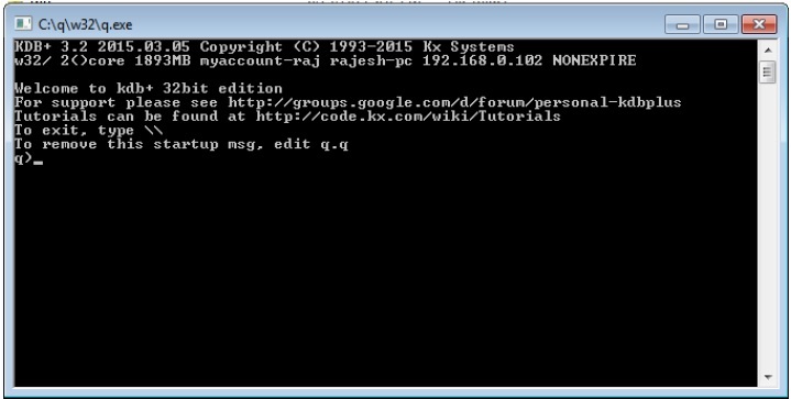
On the first line, you can see the version number which is 3.2 and the release date as 2015.03.05
Directory Layout
The trial/free version is generally installed in directories,
For linux/Mac −
~/q       / main q directory (under the user’s home)
~/q/l32   / location of linux 32-bit executable
~/q/m32   / Location of mac 32-bit executable
For Windows −
c:/q          / Main q directory
c:/q/w32/     / Location of windows 32-bit executable
Example Files −
Once you download kdb+, the directory structure in the Windows platform would appear as follows −
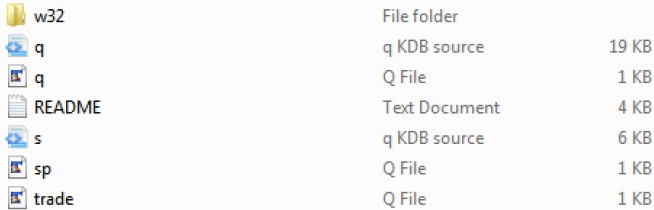
In the above directory structure, trade.q and sp.q are the example files which we can use as a reference point.
KDB+ - Architecture
Kdb+ is a high-performance, high-volume database designed from the outset to handle tremendous volumes of data. It is fully 64-bit, and has built-in multi-core processing and multi-threading. The same architecture is used for real-time and historical data. The database incorporates its own powerful query language, q, so analytics can be run directly on the data.
kdb+tick is an architecture which allows the capture, processing, and querying of real-time and historical data.
Kdb+/ tick Architecture
The following illustration provides a generalized outline of a typical Kdb+/tick architecture, followed by a brief explanation of the various components and the through-flow of data.
The Data Feeds are a time series data that are mostly provided by the data feed providers like Reuters, Bloomberg or directly from exchanges.
To get the relevant data, the data from the data feed is parsed by the feed handler.
Once the data is parsed by the feed handler, it goes to the ticker-plant.
To recover data from any failure, the ticker-plant first updates/stores the new data to the log file and then updates its own tables.
After updating the internal tables and the log files, the on-time loop data is continuously sent/published to the real-time database and all the chained subscribers who requested for data.
At the end of a business day, the log file is deleted, a new one created and the real-time database is saved onto the historical database. Once all the data is saved onto the historical database, the real-time database purges its tables.
Components of Kdb+ Tick Architecture
Data Feeds
Data Feeds can be any market or other time series data. Consider data feeds as the raw input to the feed-handler. Feeds can be directly from the exchange (live-streaming data), from the news/data providers like Thomson-Reuters, Bloomberg, or any other external agencies.
Feed Handler
A feed handler converts the data stream into a format suitable for writing to kdb+. It is connected to the data feed and it retrieves and converts the data from the feed-specific format into a Kdb+ message which is published to the ticker-plant process. Generally a feed handler is used to perform the following operations −
- Capture data according to a set of rules.
- Translate (/enrich) that data from one format to another.
- Catch the most recent values.
Ticker Plant
Ticker Plant is the most important component of KDB+ architecture. It is the ticker plant with which the real-time database or directly subscribers (clients) are connected to access the financial data. It operates in publish and subscribe mechanism. Once you obtain a subscription (license), a tick (routinely) publication from the publisher (ticker plant) is defined. It performs the following operations −
Receives the data from the feed handler.
Immediately after the ticker plant receives the data, it stores a copy as a log file and updates it once the ticker plant gets any update so that in case of any failure, we should not have any data loss.
The clients (real-time subscriber) can directly subscribe to the ticker-plant.
At the end of each business day, i.e., once the real-time database receives the last message, it stores all of today’s data onto the historical database and pushes the same to all the subscribers who have subscribed for today’s data. Then it resets all its tables. The log file is also deleted once the data is stored in the historical database or other directly linked subscriber to real time database (rtdb).
As a result, the ticker-plant, the real-time database, and the historical database are operational on a 24/7 basis.
Since the ticker-plant is a Kdb+ application, its tables can be queried using q like any other Kdb+ database. All ticker-plant clients should only have access to the database as subscribers.
Real-Time Database
A real-time database (rdb) stores today’s data. It is directly connected to the ticker plant. Typically it would be stored in memory during market hours (a day) and written out to the historical database (hdb) at the end of day. As the data (rdb data) is stored in memory, processing is extremely fast.
As kdb+ recommends to have a RAM size that is four or more times the expected size of data per day, the query that runs on rdb is very fast and provides superior performance. Since a real-time database contains only today’s data, the date column (parameter) is not required.
For example, we can have rdb queries like,
select from trade where sym = `ibm

OR

select from trade where sym = `ibm, price > 100
Historical Database
If we have to calculate the estimates of a company, we need to have its historical data available. A historical database (hdb) holds data of transactions done in the past. Each new day’s record would be added to the hdb at the end of day. Large tables in the hdb are either stored splayed (each column is stored in its own file) or they are stored partitioned by temporal data. Also some very large databases may be further partitioned using par.txt (file).
These storage strategies (splayed, partitioned, etc.) are efficient while searching or accessing the data from a large table.
A historical database can also be used for internal and external reporting purposes, i.e., for analytics. For example, suppose we want to get the company trades of IBM for a particular day from the trade (or any) table name, we need to write a query as follows −
thisday: 2014.10.12

select from trade where date = thisday, sym =`ibm
Note − We will write all such queries once we get some overview of the q language.
Q Programming Language
Kdb+ comes with its built-in programming language that is known as q. It incorporates a superset of standard SQL which is extended for time-series analysis and offers many advantages over the standard version. Anyone familiar with SQL can learn q in a matter of days and be able to quickly write her own ad-hoc queries.
Starting the “q” Environment
To start using kdb+, you need to start the q session. There are three ways to start a q session −
Simply type “c:/q/w32/q.exe” on your run terminal.
Start the MS-DOS command terminal and type q.
Copy the q.exe file onto “C:\Windows\System32” and on the run terminal, just type “q”.
Here we are assuming that you are working on a Windows platform.
Data Types
The following table provides a list of supported data types −
| Name | Example | Char | Type | Size |
|---|---|---|---|---|
| boolean | 1b | b | 1 | 1 |
| byte | 0xff | x | 4 | 1 |
| short | 23h | h | 5 | 2 |
| int | 23i | i | 6 | 4 |
| long | 23j | j | 7 | 8 |
| real | 2.3e | e | 8 | 4 |
| float | 2.3f | f | 9 | 8 |
| char | “a” | c | 10 | 1 |
| varchar | `ab | s | 11 | * |
| month | 2003.03m | m | 13 | 4 |
| date | 2015.03.17T18:01:40.134 | z | 15 | 8 |
| minute | 08:31 | u | 17 | 4 |
| second | 08:31:53 | v | 18 | 4 |
| time | 18:03:18.521 | t | 19 | 4 |
| enum | `u$`b, where u:`a`b | * | 20 | 4 |
Atom and List Formation
Atoms are single entities, e.g., a single number, a character or a symbol. In the above table (of different data types), all supported data types are atoms. A list is a sequence of atoms or other types including lists.
Passing an atom of any type to the monadic (i.e. single argument function) type function will return a negative value, i.e., –n, whereas passing a simple list of those atoms to the type function will return a positive value n.
Example 1 – Atom and List Formation
/ Note that the comments begin with a slash “ / ” and cause the parser
/ to ignore everything up to the end of the line.

x: `mohan              / `mohan is a symbol, assigned to a variable x
type x                 / let’s check the type of x
-11h                   / -ve sign, because it’s single element.

y: (`abc;`bca;`cab)    / list of three symbols, y is the variable name.

type y
11h                    / +ve sign, as it contain list of atoms (symbol).

y1: (`abc`bca`cab)     / another way of writing y, please note NO semicolon

y2: (`$”symbols may have interior blanks”)   / string to symbol conversion
y[0]                   / return `abc
y 0                    / same as y[0], also returns `abc
y 0 2                  / returns `abc`cab, same as does y[0 2]

z: (`abc; 10 20 30; (`a`b); 9.9 8.8 7.7)      / List of different types,
z 2 0                  / returns (`a`b; `abc),
z[2;0]                 / return `a. first element of z[2]

x: “Hello World!”      / list of character, a string
x 4 0                  / returns “oH” i.e. 4th and 0th(first)
element
Q Language - Type Casting
It is often required to change the data type of some data from one type to another. The standard casting function is the “$” dyadic operator.
Three approaches are used to cast from one type to another (except for string) −
- Specify desired data type by its symbol name
- Specify desired data type by its character
- Specify desired data type by it short value.
Casting Integers to Floats
In the following example of casting integers to floats, all the three different ways of casting are equivalent −
q)a:9 18 27

q)$[`float;a]     / Specify desired data type by its symbol name, 1st way
9 18 27f

q)$["f";a]        / Specify desired data type by its character, 2nd way
9 18 27f

q)$[9h;a]         / Specify desired data type by its short value, 3rd way
9 18 27f
Check if all the three operations are equivalent,
q)($[`float;a]~$["f";a]) and ($[`float;a] ~ $[9h;a])
1b
Casting Strings to Symbols
Casting string to symbols and vice versa works a bit differently. Let’s check it with an example −
q)b: ("Hello";"World";"HelloWorld")    / define a list of strings

q)b
"Hello"
"World"
"HelloWorld"

q)c: `$b                               / this is how to cast strings to symbols

q)c                                    / Now c is a list of symbols
`Hello`World`HelloWorld
Attempting to cast strings to symbols using the keyed words `symbol or 11h will fail with the type error −
q)b
"Hello"
"World"
"HelloWorld"

q)`symbol$b
'type

q)11h$b
'type
Casting Strings to Non-Symbols
Casting strings to a data type other than symbol is accomplished as follows −
q)b:900               / b contain single atomic integer

q)c:string b          / convert this integer atom to string “900”

q)c
"900"

q)`int $ c            / converting string to integer will return the
                      / ASCII equivalent of the character “9”, “0” and
                      / “0” to produce the list of integer 57, 48 and
                      / 48.
57 48 48i

q)6h $ c              / Same as above
57 48 48i

q)"i" $ c             / Same a above
57 48 48i

q)"I" $ c
900i
So to cast an entire string (the list of characters) to a single atom of data type x requires us to specify the upper case letter representing data type x as the first argument to the $ operator. If you specify the data type of x in any other way, it result in the cast being applied to each character of the string.
Q Language - Temporal Data
The q language has many different ways of representing and manipulating temporal data such as times and dates.
Date
A date in kdb+ is internally stored as the integer number of days since our reference date is 01Jan2000. A date after this date is internally stored as a positive number and a date before that is referenced as a negative number.
By default, a date is written in the format “YYYY.MM.DD”
q)x:2015.01.22      / This is how we write 22nd Jan 2015

q)`int$x            / Number of days since 2000.01.01
5500i

q)`year$x           / Extracting year from the date
2015i

q)x.year            / Another way of extracting year
2015i

q)`mm$x             / Extracting month from the date
1i

q)x.mm              / Another way of extracting month
1i

q)`dd$x             / Extracting day from the date
22i

q)x.dd              / Another way of extracting day
22i
Arithmetic and logical operations can be performed directly on dates.
q)x+1        / Add one day
2015.01.23

q)x-7        / Subtract 7 days
2015.01.15
The 1st of January 2000 fell on a Saturday. Therefore any Saturday throughout the history or in the future when divided by 7, would yield a remainder of 0, Sunday gives 1, Monday yield 2.
             Day               mod 7
           Saturday              0
           Sunday                1
           Monday                2
           Tuesday               3
           Wednesday             4
           Thursday              5
           Friday                6
Times
A time is internally stored as the integer number of milliseconds since the stroke of midnight. A time is written in the format HH:MM:SS.MSS
q)tt1: 03:30:00.000     / tt1 store the time 03:30 AM

q)tt1
03:30:00.000

q)`int$tt1              / Number of milliseconds in 3.5 hours
12600000i

q)`hh$tt1               / Extract the hour component from time
3i

q)tt1.hh
3i

q)`mm$tt1               / Extract the minute component from time
30i

q)tt1.mm
30i

q)`ss$tt1               / Extract the second component from time
0i

q)tt1.ss
0i
As in case of dates, arithmetic can be performed directly on times.
Datetimes
A datetime is the combination of a date and a time, separated by ‘T’ as in the ISO standard format. A datetime value stores the fractional day count from midnight Jan 1, 2000.
q)dt:2012.12.20T04:54:59:000      / 04:54.59 AM on 20thDec2012

q)type dt
-15h

q)dt
2012.12.20T04:54:59.000
9
q)`float$dt
4737.205
The underlying fractional day count can be obtained by casting to float.
Q Language - Lists
Lists are the basic building blocks of q language, so a thorough understanding of lists is very important. A list is simply an ordered collection of atoms (atomic elements) and other lists (group of one or more atoms).
Types of List
A general list encloses its items within matching parentheses and separates them with semicolons. For example −
(9;8;7) or ("a"; "b"; "c") or (-10.0; 3.1415e; `abcd; "r")
If a list comprises of atoms of same type, it is known as a uniform list. Else, it is known as a general list (mixed type).
Count
We can obtain the number of items in a list through its count.
q)l1:(-10.0;3.1415e;`abcd;"r")    / Assigning variable name to general list

q)count l1                        / Calculating number of items in the list l1
4
Examples of simple List
q)h:(1h;2h;255h)                    / Simple Integer List

q)h
1 2 255h

q)f:(123.4567;9876.543;98.7)        / Simple Floating Point List

q)f
123.4567 9876.543 98.7

q)b:(0b;1b;0b;1b;1b)                / Simple Binary Lists

q)b
01011b

q)symbols:(`Life;`Is;`Beautiful)    / Simple Symbols List

q)symbols
`Life`Is`Beautiful

q)chars:("h";"e";"l";"l";"o";" ";"w";"o";"r";"l";"d")
                                    / Simple char lists and Strings.
q)chars
"hello world"
**Note − A simple list of char is called a string.
A list contains atoms or lists. To create a single item list, we use −
q)singleton:enlist 42

q)singleton
,42
To distinguish between an atom and the equivalent singleton, examine the sign of their type.
q)signum type 42
-1i

q)signum type enlist 42
1i
Q Language - Indexing
A list is ordered from left to right by the position of its items. The offset of an item from the beginning of the list is called its index. Thus, the first item has an index 0, the second item (if there is one) has an index 1, etc. A list of count n has index domain from 0 to n–1.
Index Notation
Given a list L, the item at index i is accessed by L[i]. Retrieving an item by its index is called item indexing. For example,
q)L:(99;98.7e;`b;`abc;"z")

q)L[0]
99

q)L[1]
98.7e

q)L[4]
"z
Indexed Assignment
Items in a list can also be assigned via item indexing. Thus,
q)L1:9 8 7

q)L1[2]:66      / Indexed assignment into a simple list
                / enforces strict type matching.

q)L1
9 8 66
Lists from Variables
q)l1:(9;8;40;200)

q)l2:(1 4 3; `abc`xyz)

q)l:(l1;l2)               / combining the two list l1 and l2

q)l
9 8 40 200
(1 4 3;`abc`xyz)
Joining Lists
The most common operation on two lists is to join them together to form a larger list. More precisely, the join operator (,) appends its right operand to the end of the left operand and returns the result. It accepts an atom in either argument.
q)1,2 3 4
1 2 3 4

q)1 2 3, 4.4 5.6     / If the arguments are not of uniform type,
                     / the result is a general list.
1
2
3
4.4
5.6
Nesting
Data complexity is built by using lists as items of lists.
Depth
The number of levels of nesting for a list is called its depth. Atoms have a depth of 0 and simple lists have a depth of 1.
q)l1:(9;8;(99;88))

q)count l1
3
Here is a list of depth 3 having two items −
q)l5
9
(90;180;900 1800 2700 3600)

q)count l5
2

q)count l5[1]
3
Indexing at Depth
It is possible to index directly into the items of a nested list.
Repeated Item Indexing
Retrieving an item via a single index always retrieves an uppermost item from a nested list.
q)L:(1;(100;200;(300;400;500;600)))

q)L[0]
1

q)L[1]
100
200
300 400 500 600
Since the result L[1] is itself a list, we can retrieve its elements using a single index.
q)L[1][2]
300 400 500 600
We can repeat single indexing once more to retrieve an item from the innermost nested list.
q)L[1][2][0]
300
You can read this as,
Get the item at index 1 from L, and from it retrieve the item at index 2, and from it retrieve the item at index 0.
Notation for Indexing at Depth
There is an alternate notation for repeated indexing into the constituents of a nested list. The last retrieval can also be written as,
q)L[1;2;0]
300
Assignment via index also works at depth.
q)L[1;2;1]:900

q)L
1
(100;200;300 900 500 600)
Elided Indices
Eliding Indices for a General List
q)L:((1 2 3; 4 5 6 7); (`a`b`c;`d`e`f`g;`0`1`2);("good";"morning"))

q)L
(1 2 3;4 5 6 7)
(`a`b`c;`d`e`f`g;`0`1`2)
("good";"morning")

q)L[;1;]
4 5 6 7
`d`e`f`g
"morning"

q)L[;;2]
3 6
`c`f`2
"or"
Interpret L[;1;] as,
Retrieve all items in the second position of each list at the top level.
Interpret L[;;2] as,
Retrieve the items in the third position for each list at the second level.
Q Language - Dictionaries
Dictionaries are an extension of lists which provide the foundation for creating tables. In mathematical terms, dictionary creates the
“domain → Range”
or in general (short) creates
“key → value”
relationship between elements.
A dictionary is an ordered collection of key-value pairs that is roughly equivalent to a hash table. A dictionary is a mapping defined by an explicit I/O association between a domain list and a range list via positional correspondence. The creation of a dictionary uses the "xkey" primitive (!)
ListOfDomain ! ListOfRange
The most basic dictionary maps a simple list to a simple list.
| Input (I) | Output (O) |
|---|---|
| `Name | `John |
| `Age | 36 |
| `Sex | “M” |
| Weight | 60.3 |
q)d:`Name`Age`Sex`Weight!(`John;36;"M";60.3)   / Create a dictionary d

q)d

Name   | `John
Age    | 36
Sex    | "M"
Weight | 60.3

q)count d             / To get the number of rows in a dictionary.
4

q)key d               / The function key returns the domain
`Name`Age`Sex`Weight

q)value d             / The function value returns the range.

`John
36

"M"
60.3

q)cols d             / The function cols also returns the domain.
`Name`Age`Sex`Weight
Lookup
Finding the dictionary output value corresponding to an input value is called looking up the input.
q)d[`Name]       / Accessing the value of domain `Name
`John

q)d[`Name`Sex]   / extended item-wise to a simple list of keys
`John
"M"
Lookup with Verb @
q)d1:`one`two`three!9 18 27

q)d1[`two]
18

q)d1@`two
18
Operations on Dictionaries
Amend and Upsert
As with lists, the items of a dictionary can be modified via indexed assignment.
d:`Name`Age`Sex`Weight! (`John;36;"M";60.3)
                                  / A dictionary d

q)d[`Age]:35                      / Assigning new value to key Age

q)d
                              / New value assigned to key Age in d
Name   | `John
Age    | 35
Sex    | "M"
Weight | 60.3
Dictionaries can be extended via index assignment.
q)d[`Height]:"182 Ft"

q)d

Name   | `John
Age    | 35
Sex    | "M"
Weight | 60.3
Height | "182 Ft"
Reverse Lookup with Find (?)
The find (?) operator is used to perform reverse lookup by mapping a range of elements to its domain element.
q)d2:`x`y`z!99 88 77

q)d2?77
`z
In case the elements of a list is not unique, the find returns the first item mapping to it from the domain list.
Removing Entries
To remove an entry from a dictionary, the delete ( _ ) function is used. The left operand of ( _ ) is the dictionary and the right operand is a key value.
q)d2:`x`y`z!99 88 77

q)d2 _`z

x| 99
y| 88
Whitespace is required to the left of _ if the first operand is a variable.
q)`x`y _ d2           / Deleting multiple entries

z| 77
Column Dictionaries
Column dictionaries are the basics for creation of tables. Consider the following example −
q)scores: `name`id!(`John`Jenny`Jonathan;9 18 27)
                              / Dictionary scores

q)scores[`name]               / The values for the name column are
`John`Jenny`Jonathan

q)scores.name                 / Retrieving the values for a column in a
                              / column dictionary using dot notation.
`John`Jenny`Jonathan

q)scores[`name][1]            / Values in row 1 of the name column
`Jenny

q)scores[`id][2]              / Values in row 2 of the id column is
27
Flipping a Dictionary
The net effect of flipping a column dictionary is simply reversing the order of the indices. This is logically equivalent to transposing the rows and columns.
Flip on a Column Dictionary
The transpose of a dictionary is obtained by applying the unary flip operator. Take a look at the following example −
q)scores

name  | John Jenny Jonathan
id    | 9   18   27

q)flip scores

  name     id
---------------
  John     9
  Jenny    18
 Jonathan  27
Flip of a Flipped Column Dictionary
If you transpose a dictionary twice, you obtain the original dictionary,
q)scores ~ flip flip scores
1b
Q Language - Table
Tables are at the heart of kdb+. A table is a collection of named columns implemented as a dictionary. q tables are column-oriented.
Creating Tables
Tables are created using the following syntax −
q)trade:([]time:();sym:();price:();size:())

q)trade
time sym price size
-------------------
In the above example, we have not specified the type of each column. This will be set by the first insert into the table.
Another way, we can specify column type on initialization −
q)trade:([]time:`time$();sym:`$();price:`float$();size:`int$())
Or we can also define non-empty tables −
q)trade:([]sym:(`a`b);price:(1 2))

q)trade

 sym   price
-------------
  a      1
  b      2
If there are no columns within the square brackets as in the examples above, the table is unkeyed.
To create a keyed table, we insert the column(s) for the key in the square brackets.
q)trade:([sym:`$()]time:`time$();price:`float$();size:`int$())

q)trade

 sym   | time price size
-----  | ---------------
One can also define the column types by setting the values to be null lists of various types −
q)trade:([]time:0#0Nt;sym:0#`;price:0#0n;size:0#0N)
Getting Table Information
Let’s create a trade table −
trade: ([]sym:`ibm`msft`apple`samsung;mcap:2000 4000 9000 6000;ex:`nasdaq`nasdaq`DAX`Dow)

q)cols trade                         / column names of a table
`sym`mcap`ex

q)trade.sym                          / Retrieves the value of column sym
`ibm`msft`apple`samsung

q)show meta trade                    / Get the meta data of a table trade.

  c   | t f a
----- | -----
 Sym  | s
 Mcap | j
 ex   | s
Primary Keys and Keyed Tables
Keyed Table
A keyed table is a dictionary that maps each row in a table of unique keys to a corresponding row in a table of values. Let us take an example −
val:flip `name`id!(`John`Jenny`Jonathan;9 18 27)
                          / a flip dictionary create table val
id:flip (enlist `eid)!enlist 99 198 297
                          / flip dictionary, having single column eid
Now create a simple keyed table containing eid as key,
q)valid: id ! val

q)valid                 / table name valid, having key as eid

  eid |  name      id
---   | ---------------
  99  |  John      9
  198 |  Jenny     18
  297 |  Jonathan  27
ForeignKeys
A foreign key defines a mapping from the rows of the table in which it is defined to the rows of the table with the corresponding primary key.
Foreign keys provide referential integrity. In other words, an attempt to insert a foreign key value that is not in the primary key will fail.
Consider the following examples. In the first example, we will define a foreign key explicitly on initialization. In the second example, we will use foreign key chasing which does not assume any prior relationship between the two tables.
Example 1 − Define foreign key on initialization
q)sector:([sym:`SAMSUNG`HSBC`JPMC`APPLE]ex:`N`CME`DAQ`N;MC:1000 2000 3000 4000)

q)tab:([]sym:`sector$`HSBC`APPLE`APPLE`APPLE`HSBC`JPMC;price:6?9f)

q)show meta tab

  c    | t f a
------ | ----------
 sym   | s sector
 price | f

q)show select from tab where sym.ex=`N

  sym     price
----------------
 APPLE   4.65382
 APPLE   4.643817
 APPLE   3.659978
Example 2 − no pre-defined relationship between tables
sector: ([symb:`IBM`MSFT`HSBC]ex:`N`CME`N;MC:1000 2000 3000)
tab:([]sym:`IBM`MSFT`MSFT`HSBC`HSBC;price:5?9f)
To use foreign key chasing, we must create a table to key into sector.
q)show update mc:(sector([]symb:sym))[`MC] from tab

  sym     price      mc
--------------------------
  IBM   7.065297    1000
  MSFT  4.812387    2000
  MSFT  6.400545    2000
  HSBC  3.704373    3000
  HSBC  4.438651    3000
General notation for a predefined foreign key −
select a.b from c where a is the foreign key (sym), b is a
field in the primary key table (ind), c is the
foreign key table (trade)
Manipulating Tables
Let’s create one trade table and check the result of different table expression −
q)trade:([]sym:5?`ibm`msft`hsbc`samsung;price:5?(303.00*3+1);size:5?(900*5);time:5?(.z.T-365))

q)trade

  sym        price   size   time
-----------------------------------------
 msft      743.8592  3162  02:32:17.036
 msft      641.7307  2917  01:44:56.936
 hsbc      838.2311  1492  00:25:23.210
 samsung   278.3498  1983  00:29:38.945
 ibm       838.6471  4006  07:24:26.842
Let us now take a look at the statements that are used to manipulate tables using q language.
Select
The syntax to use a Select statement is as follows −
select [columns] [by columns] from table [where clause]
Let us now take an example to demonstrate how to use Select statement −
q)/ select expression example

q)select sym,price,size by time from trade where size > 2000

    time      |  sym    price     size
------------- | -----------------------
 01:44:56.936 |  msft   641.7307  2917
 02:32:17.036 |  msft   743.8592  3162
 07:24:26.842 |  ibm    838.6471  4006
Insert
The syntax to use an Insert statement is as follows −
`tablename insert (values)
Insert[`tablename; values]
Let us now take an example to demonstrate how to use Insert statement −
q)/ Insert expression example

q)`trade insert (`hsbc`apple;302.0 730.40;3020 3012;09:30:17.00409:15:00.000)
5 6

q)trade

   sym    price     size    time
------------------------------------------
  msft    743.8592  3162   02:32:17.036
  msft    641.7307  2917   01:44:56.936
  hsbc    838.2311  1492   00:25:23.210
 samsung  278.3498  1983   00:29:38.945
  ibm     838.6471  4006   07:24:26.842
  hsbc    302       3020   09:30:17.004
  apple   730.4     3012   09:15:00.000

q)/Insert another value

q)insert[`trade;(`samsung;302.0; 3333;10:30:00.000]
']

q)insert[`trade;(`samsung;302.0; 3333;10:30:00.000)]
,7

q)trade

   sym     price   size     time
----------------------------------------
  msft   743.8592  3162  02:32:17.036
  msft   641.7307  2917  01:44:56.936
  hsbc   838.2311  1492  00:25:23.210
 samsung 278.3498  1983  00:29:38.945
  ibm    838.6471  4006  07:24:26.842
  hsbc   302       3020  09:30:17.004
  apple  730.4     3012  09:15:00.000
 samsung 302       3333  10:30:00.000
Delete
The syntax to use a Delete statement is as follows −
delete columns from table
delete from table where clause
Let us now take an example to demonstrate how to use Delete statement −
q)/Delete expression example

q)delete price from trade

   sym   size       time
-------------------------------
  msft   3162   02:32:17.036
  msft   2917   01:44:56.936
  hsbc   1492   00:25:23.210
 samsung 1983   00:29:38.945
  ibm    4006   07:24:26.842
  hsbc   3020   09:30:17.004
  apple  3012   09:15:00.000
 samsung 3333   10:30:00.000

q)delete from trade where price > 3000

   sym     price     size       time
-------------------------------------------
  msft    743.8592   3162    02:32:17.036
  msft    641.7307   2917    01:44:56.936
  hsbc    838.2311   1492    00:25:23.210
 samsung  278.3498   1983    00:29:38.945
  ibm     838.6471   4006    07:24:26.842
  hsbc    302        3020    09:30:17.004
  apple   730.4      3012    09:15:00.000
 samsung  302        3333    10:30:00.000

q)delete from trade where price > 500

  sym     price     size     time
-----------------------------------------
 samsung  278.3498  1983  00:29:38.945
  hsbc    302       3020  09:30:17.004
 samsung  302       3333  10:30:00.000
Update
The syntax to use an Update statement is as follows −
update column: newValue from table where ….
Use the following syntax to update the format/datatype of a column using the cast function −
update column:newValue from `table where …
Let us now take an example to demonstrate how to use Update statement −
q)/Update expression example

q)update size:9000 from trade where price > 600

  sym     price      size     time
------------------------------------------
  msft    743.8592   9000   02:32:17.036
  msft    641.7307   9000   01:44:56.936
  hsbc    838.2311   9000   00:25:23.210
 samsung  278.3498   1983   00:29:38.945
  ibm     838.6471   9000   07:24:26.842
  hsbc    302        3020   09:30:17.004
  apple   730.4      9000   09:15:00.000
 samsung  302        3333   10:30:00.000

q)/Update the datatype of a column using the cast function

q)meta trade

   c  |  t f a
----- | --------
  sym |  s
 price|  f
 size |  j
 time |  t

q)update size:`float$size from trade

  sym     price     size      time
------------------------------------------
  msft    743.8592  3162    02:32:17.036
  msft    641.7307  2917    01:44:56.936
  hsbc    838.2311  1492    00:25:23.210
 samsung  278.3498  1983    00:29:38.945
  ibm     838.6471  4006    07:24:26.842
  hsbc    302       3020    09:30:17.004
  apple   730.4     3012    09:15:00.000
 samsung  302       3333    10:30:00.000

q)/ Above statement will not update the size column datatype permanently

q)meta trade

   c   |  t f a
------ | --------
  sym  |   s
 price |   f
 size  |   j
 time  |   t

q)/to make changes in the trade table permanently, we have do

q)update size:`float$size from `trade
`trade

q)meta trade

   c   |  t f a
------ | --------
  sym  |   s
 price |   f
 size  |   f
 time  |   t
Q Language - Verb & Adverbs
Kdb+ has nouns, verbs, and adverbs. All data objects and functions are nouns. Verbs enhance the readability by reducing the number of square brackets and parentheses in expressions. Adverbs modify dyadic (2 arguments) functions and verbs to produce new, related verbs. The functions produced by adverbs are called derived functions or derived verbs.
Each
The adverb each, denoted by ( ` ), modifies dyadic functions and verbs to apply to the items of lists instead of the lists themselves. Take a look at the following example −
q)1, (2 3 5)       / Join
1 2 3 5

q)1, '( 2 3 4)     / Join each
1 2
1 3
1 4
There is a form of Each for monadic functions that uses the keyword “each”. For example,
q)reverse ( 1 2 3; "abc")           /Reverse
a b c
1 2 3

q)each [reverse] (1 2 3; "abc")     /Reverse-Each
3 2 1
c b a

q)'[reverse] ( 1 2 3; "abc")
3 2 1
c b a
Each-Left and Each-Right
There are two variants of Each for dyadic functions called Each-Left (\:) and Each-Right (/:). The following example explains how to use them.
q)x: 9 18 27 36

q)y:10 20 30 40

q)x,y            / join
9 18 27 36 10 20 30 40

q)x,'y           / each

9   10
18  20
27  30
36  40

q)x: 9 18 27 36

q)y:10 20 30 40

q)x,y            / join
9 18 27 36 10 20 30 40

q)x,'y           / each, will return a list of pairs

9   10
18  20
27  30
36  40

q)x, \:y         / each left, returns a list of each element
                 / from x with all of y

9   10  20  30  40
18  10  20  30  40
27  10  20  30  40
36  10  20  30  40

q)x,/:y          / each right, returns a list of all the x with
                 / each element of y

9  18  27  36  10
9  18  27  36  20
9  18  27  36  30
9  18  27  36  40

q)1 _x           / drop the first element
18 27 36

q)-2_y           / drop the last two element
10 20

q)               / Combine each left and each right to be a
                 / cross-product (cartesian product)

q)x,/:\:y

9   10  9   20  9   30  9   40
18  10  18  20  18  30  18  40
27  10  27  20  27  30  27  40
36  10  36  20  36  30  36  40
Q Language - Joins
In q language, we have different kinds of joins based on the input tables supplied and the kind of joined tables we desire. A join combines data from two tables. Besides foreign key chasing, there are four other ways to join tables −
- Simple join
- Asof join
- Left join
- Union join
Here, in this chapter, we will discuss each of these joins in detail.
Simple Join
Simple join is the most basic type of join, performed with a comma ‘,’. In this case, the two tables have to be type conformant, i.e., both the tables have the same number of columns in the same order, and same key.
table1,:table2 / table1 is assigned the value of table2
We can use comma-each join for tables with same length to join sideways. One of the tables can be keyed here,
Table1, `Table2
Asof Join (aj)
It is the most powerful join which is used to get the value of a field in one table asof the time in another table. Generally it is used to get the prevailing bid and ask at the time of each trade.
General format
aj[joinColumns;tbl1;tbl2]
For example,
aj[`sym`time;trade;quote]
Example
q)tab1:([]a:(1 2 3 4);b:(2 3 4 5);d:(6 7 8 9))

q)tab2:([]a:(2 3 4);b:(3 4 5); c:( 4 5 6))

q)show aj[`a`b;tab1;tab2]

 a  b  d  c
-------------
 1  2  6
 2  3  7  4
 3  4  8  5
 4  5  9  6
Left Join(lj)
It’s a special case of aj where the second argument is a keyed table and the first argument contains the columns of the right argument’s key.
General format
table1 lj Keyed-table
Example
q)/Left join- syntax table1 lj table2 or lj[table1;table2]

q)tab1:([]a:(1 2 3 4);b:(2 3 4 5);d:(6 7 8 9))

q)tab2:([a:(2 3 4);b:(3 4 5)]; c:( 4 5 6))

q)show lj[tab1;tab2]

 a  b  d  c
-------------
 1  2  6
 2  3  7  4
 3  4  8  5
 4  5  9  6
Union Join (uj)
It allows to create a union of two tables with distinct schemas. It is basically an extension to the simple join ( , )
q)tab1:([]a:(1 2 3 4);b:(2 3 4 5);d:(6 7 8 9))

q)tab2:([]a:(2 3 4);b:(3 4 5); c:( 4 5 6))

q)show uj[tab1;tab2]

 a  b  d  c
------------
 1  2  6
 2  3  7
 3  4  8
 4  5  9
 2  3     4
 3  4     5
 4  5     6
If you are using uj on keyed tables, then the primary keys must match.
Q Language - Functions
Types of Functions
Functions can be classified in a number of ways. Here we have classified them based on the number and type of argument they take and the result type. Functions can be,
Atomic − Where the arguments are atomic and produce atomic results
Aggregate − atom from list
Uniform (list from list) − Extended the concept of atom as they apply to lists. The count of the argument list equals the count of the result list.
Other − if the function is not from the above category.
Binary operations in mathematics are called dyadic functions in q; for example, “+”. Similarly unary operations are called monadic functions; for example, “abs” or “floor”.
Frequently Used Functions
There are quite a few functions used frequently in q programming. Here, in this section, we will see the usage of some popular functions −
abs
q) abs -9.9 / Absolute value, Negates -ve number & leaves non -ve number
9.9
all
q) all 4 5 0 -4 / Logical AND (numeric min), returns the minimum value
0b
Max (&), Min (|), and Not (!)
q) /And, Or, and Logical Negation

q) 1b & 1b        / And (Max)
1b

q) 1b|0b              / Or (Min)
1b

q) not 1b             /Logical Negate (Not)
0b
asc
q)asc 1 3 5 7 -2 0 4    / Order list ascending, sorted list
                        / in ascending order i
s returned
`s#-2 0 1 3 4 5 7

q)/attr - gives the attributes of data, which describe how it's sorted.
`s denotes fully sorted, `u denotes unique and `p and `g are used to
refer to lists with repetition, with `p standing for parted and `g for grouped
avg
q)avg 3 4 5 6 7           / Return average of a list of numeric values
5f

q)/Create on trade table

q)trade:([]time:3?(.z.Z-200);sym:3?(`ibm`msft`apple);price:3?99.0;size:3?100)
by
q)/ by - Groups rows in a table at given sym

q)select sum price by sym from trade    / find total price for each sym

  sym  |   price
------ | --------
 apple | 140.2165
  ibm  | 16.11385
cols
q)cols trade / Lists columns of a table
`time`sym`price`size
count
q)count (til 9) / Count list, count the elements in a list and
                / return a single int value 9
port
q)\p 9999 / assign port number

q)/csv - This command allows queries in a browser to be exported to
   excel by prefixing the query, such as http://localhost:9999/.csv?select from trade where sym =`ibm
cut
q)/ cut - Allows a table or list to be cut at a certain point

q)(1 3 5) cut "abcdefghijkl"
                            / the argument is split at 1st, 3rd and 5th letter.
"bc"
"de"
"fghijkl"

q)5 cut "abcdefghijkl"      / cut the right arg. Into 5 letters part
                            / until its end.
"abcde"
"fghij"
"kl"
Delete
q)/delete - Delete rows/columns from a table

q)delete price from trade

          time              sym   size
---------------------------------------
  2009.06.18T06:04:42.919  apple   36
  2009.11.14T12:42:34.653   ibm    12
  2009.12.27T17:02:11.518  apple   97
Distinct
q)/distinct - Returns the distinct element of a list

q)distinct 1 2 3 2 3 4 5 2 1 3            / generate unique set of number
1 2 3 4 5
enlist
q)/enlist - Creates one-item list.

q)enlist 37
,37

q)type 37           / -ve type value
-7h

q)type enlist 37    / +ve type value
7h
Fill (^)
q)/fill - used with nulls. There are three functions for processing null values.

The dyadic function named fill replaces null values in the right argument with the atomic left argument.

q)100 ^ 3 4 0N 0N -5
3 4 100 100 -5

q)`Hello^`jack`herry``john`
`jack`herry`Hello`john`Hello
Fills
q)/fills - fills in nulls with the previous not null value.

q)fills 1 0N 2 0N 0N 2 3 0N -5 0N
1 1 2 2 2 2 3 3 -5 -5
First
q)/first - returns the first atom of a list

q)first 1 3 34 5 3
1
Flip
q)/flip - Monadic primitive that applies to lists and associations. It interchange the top two levels of its argument.

q)trade

       time                   sym      price   size
------------------------------------------------------
  2009.06.18T06:04:42.919    apple   72.05742   36
  2009.11.14T12:42:34.653    ibm     16.11385   12
  2009.12.27T17:02:11.518    apple   68.15909   97

q)flip trade

time | 2009.06.18T06:04:42.919 2009.11.14T12:42:34.653
2009.12.27T17:02:11.518

sym   |  apple         ibm         apple
price | 72.05742     16.11385    68.15909
size  | 36 12 97
iasc
q)/iasc - Index ascending, return the indices of the ascended sorted list relative to the input list.

q)iasc 5 4 0 3 4 9

2 3 1 4 0 5
Idesc
q)/idesc - Index desceding, return the descended sorted list relative to the input list

q)idesc 0 1 3 4

3 2 1 0
in
q)/in - In a list, dyadic function used to query list (on the right-handside) about their contents.

q)(2 4) in 1 2 3

10b
insert
q)/insert - Insert statement, upload new data into a table.

q)insert[`trade;((.z.Z);`samsung;48.35;99)],3

q)trade

      time                  sym       price     size
------------------------------------------------------
 2009.06.18T06:04:42.919   apple    72.05742     36
 2009.11.14T12:42:34.653    ibm     16.11385     12
 2009.12.27T17:02:11.518   apple    68.15909     97
 2015.04.06T10:03:36.738   samsung  48.35        99
key
q)/key - three different functions i.e. generate +ve integer number, gives content of a directory or key of a table/dictionary.

q)key 9

0 1 2 3 4 5 6 7 8

q)key `:c:
`$RECYCLE.BIN`Config.Msi`Documents and Settings`Drivers`Geojit`hiberfil.sys`I..
lower
q)/lower - Convert to lower case and floor

q)lower ("JoHn";`HERRY`SYM)
"john"
`herry`sym
Max and Min (i.e. | and &)
q)/Max and Min / a|b and a&b

q)9|7
9

q)9&5
5
null
q)/null - return 1b if the atom is a null else 0b from the argument list

q)null 1 3 3 0N
0001b
Peach
q)/peach - Parallel each, allows process across slaves

q)foo peach list1       / function foo applied across the slaves named in list1

'list1

q)foo:{x+27}

q)list1:(0 1 2 3 4)

q)foo peach list1       / function foo applied across the slaves named in list1
27 28 29 30 31
Prev
q)/prev - returns the previous element i.e. pushes list forwards

q)prev 0 1 3 4 5 7

0N 0 1 3 4 5
Random( ?)
q)/random - syntax - n?list, gives random sequences of ints and floats

q)9?5
0 0 4 0 3 2 2 0 1

q)3?9.9
0.2426823 1.674133 3.901671
Raze
q)/raze - Flattn a list of lists, removes a layer of indexing from a list of lists. for instance:

q)raze (( 12 3 4; 30 0);("hello";7 8); 1 3 4)

12 3 4
30 0
"hello"
7 8
1
3
4
read0
q)/read0 - Read in a text file

q)read0 `:c:/q/README.txt    / gives the contents of *.txt file
read1
q)/read1 - Read in a q data file

q)read1 `:c:/q/t1

0xff016200630b000500000073796d0074696d6500707269636…
reverse
q)/reverse - Reverse a list

q)reverse 2 30 29 1 3 4

4 3 1 29 30 2

q)reverse "HelloWorld"

"dlroWolleH"
set
q)/set - set value of a variable

q)`x set 9
`x

q)x
9

q)`:c:/q/test12 set trade

`:c:/q/test12

q)get `:c:/q/test12

       time                   sym      price     size
---------------------------------------------------------
  2009.06.18T06:04:42.919    apple    72.05742    36
  2009.11.14T12:42:34.653     ibm     16.11385    12
  2009.12.27T17:02:11.518    apple    68.15909    97
  2015.04.06T10:03:36.738    samsung  48.35       99
  2015.04.06T10:03:47.540    samsung  48.35       99
  2015.04.06T10:04:44.844    samsung  48.35       99
ssr
q)/ssr - String search and replace, syntax - ssr["string";searchstring;replaced-with]

q)ssr["HelloWorld";"o";"O"]

"HellOWOrld"
string
q)/string - converts to string, converts all types to a string format.

q)string (1 2 3; `abc;"XYZ";0b)

(,"1";,"2";,"3")
"abc"

(,"X";,"Y";,"Z")
,"0"
SV
q)/sv - Scalar from vector, performs different tasks dependent on its arguments.

It evaluates the base representation of numbers, which allows us to calculate the number of seconds in a month or convert a length from feet and inches to centimeters.

q)24 60 60 sv 11 30 49

41449   / number of seconds elapsed in a day at 11:30:49
system
q)/system - allows a system command to be sent,

q)system "dir *.py"

" Volume in drive C is New Volume"
" Volume Serial Number is 8CD2-05B2"
""

" Directory of C:\\Users\\myaccount-raj"
""

"09/14/2014    06:32 PM     22 hello1.py"
"                1 File(s)    22 bytes"
tables
q)/tables - list all tables

q)tables `

`s#`tab1`tab2`trade
Til
q)/til - Enumerate

q)til 5

0 1 2 3 4
trim
q)/trim - Eliminate string spaces

q)trim " John "

"John"
vs
q)/vs - Vector from scaler , produces a vector quantity from a scaler quantity

q)"|" vs "20150204|msft|20.45"

"20150204"
"msft"
"20.45"
xasc
q)/xasc - Order table ascending, allows a table (right-hand argument) to be sorted such that (left-hand argument) is in ascending order

q)`price xasc trade

          time                 sym      price      size
----------------------------------------------------------
   2009.11.14T12:42:34.653     ibm     16.11385     12
   2015.04.06T10:03:36.738   samsung   48.35        99
   2015.04.06T10:03:47.540   samsung   48.35        99
   2015.04.06T10:04:44.844   samsung   48.35        99
   2009.12.27T17:02:11.518    apple    68.15909     97
   2009.06.18T06:04:42.919    apple    72.05742     36
xcol
q)/xcol - Renames columns of a table

q)`timeNew`symNew xcol trade

        timeNew                 symNew    price      size
-------------------------------------------------------------
   2009.06.18T06:04:42.919      apple    72.05742     36
   2009.11.14T12:42:34.653       ibm     16.11385     12
   2009.12.27T17:02:11.518      apple    68.15909     97
   2015.04.06T10:03:36.738     samsung   48.35        99
   2015.04.06T10:03:47.540     samsung   48.35        99
   2015.04.06T10:04:44.844     samsung   48.35        99
xcols
q)/xcols - Reorders the columns of a table,

q)`size`price xcols trade

  size    price           time                   sym
-----------------------------------------------------------
   36   72.05742   2009.06.18T06:04:42.919      apple
   12   16.11385   2009.11.14T12:42:34.653       ibm
   97   68.15909   2009.12.27T17:02:11.518      apple
   99   48.35      2015.04.06T10:03:36.738     samsung
   99   48.35      2015.04.06T10:03:47.540     samsung
   99   48.35      2015.04.06T10:04:44.844     samsung
xdesc
q)/xdesc - Order table descending, allows tables to be sorted such that the left-hand argument is in descending order.

q)`price xdesc trade

        time                   sym       price      size
-----------------------------------------------------------
   2009.06.18T06:04:42.919    apple    72.05742      36
   2009.12.27T17:02:11.518    apple    68.15909      97
   2015.04.06T10:03:36.738   samsung   48.35         99
   2015.04.06T10:03:47.540   samsung   48.35         99
   2015.04.06T10:04:44.844   samsung   48.35         99
   2009.11.14T12:42:34.653     ibm     16.11385      12
xgroup
q)/xgroup - Creates nested table

q)`x xgroup ([]x:9 18 9 18 27 9 9;y:10 20 10 20 30 40)
'length

q)`x xgroup ([]x:9 18 9 18 27 9 9;y:10 20 10 20 30 40 10)

  x  |    y
---- | -----------
  9  | 10 10 40 10
  18 | 20 20
  27 | ,30
xkey
q)/xkey - Set key on table

q)`sym xkey trade

    sym   |      time                    price     size
--------- | -----------------------------------------------
   apple  | 2009.06.18T06:04:42.919    72.05742     36
    ibm   | 2009.11.14T12:42:34.653    16.11385     12
   apple  | 2009.12.27T17:02:11.518    68.15909     97
  samsung | 2015.04.06T10:03:36.738    48.35        99
  samsung | 2015.04.06T10:03:47.540    48.35        99
  samsung | 2015.04.06T10:04:44.844    48.35        99
System Commands
System commands control the q environment. They are of the following form −
\cmd [p] where p may be optional
Some of the popular system commands have been discussed below −
\a [ namespace] – List tables in the given namespace
q)/Tables in default namespace

q)\a
,`trade

q)\a .o         / table in .o namespace.
,`TI
\b – View dependencies
q)/ views/dependencies

q)a:: x+y      / global assingment

q)b:: x+1

q)\b
`s#`a`b
\B – Pending views / dependencies
q)/ Pending views/dependencies

q)a::x+1     / a depends on x

q)\B         / the dependency is pending
' / the dependency is pending

q)\B
`s#`a`b

q)\b
`s#`a`b

q)b
29

q)a
29

q)\B
`symbol$()
\cd – Change directory
q)/change directory, \cd [name]

q)\cd
"C:\\Users\\myaccount-raj"

q)\cd ../new-account

q)\cd
"C:\\Users\\new-account"
\d – sets current namespace
q)/ sets current namespace \d [namespace]

q)\d             /default namespace
'

q)\d .o          /change to .o

q.o)\d
`.o

q.o)\d .         / return to default

q)key `          /lists namespaces other than .z
`q`Q`h`j`o

q)\d .john       /change to non-existent namespace

q.john)\d
`.john

q.john)\d .

q)\d
`.
\l – load file or directory from db
q)/ Load file or directory, \l

q)\l test2.q / loading test2.q which is stored in current path.

   ric      |     date      ex      openP    closeP    MCap
----------- | -------------------------------------------------
 JPMORGAN   | 2008.05.23  SENSEX  18.30185  17.16319  17876
   HSBC     | 2002.05.21  NIFTY   2.696749  16.58846  26559
 JPMORGAN   | 2006.09.07  NIFTY   14.15219  20.05624  14557
   HSBC     | 2010.10.11  SENSEX  7.394497  25.45859  29366
 JPMORGAN   | 2007.10.02  SENSEX  1.558085  25.61478  20390

   ric     |    date       ex      openP     closeP    MCap
---------- | ------------------------------------------------
  INFOSYS  | 2003.10.30    DOW    21.2342   7.565652   2375
 RELIANCE  | 2004.08.12    DOW    12.34132  17.68381   4201
   SBIN    | 2008.02.14    DOW    1.830857  9.006485   15465
  INFOSYS  | 2009.06.11  HENSENG  19.47664  12.05208   11143
   SBIN    | 2010.07.05    DOW    18.55637  10.54082   15873
\p – port number
q)/ assign port number, \p

q)\p
5001i

q)\p 8888

q)\p
8888i
\\ - Exit from q console
\\ - exit
Exit form q.
Q Language - Built-in Functions
The q programming language has a set of rich and powerful built-in functions. A built-in function can be of the following types −
String function − Takes a string as input and returns a string.
Aggregate function − Takes a list as input and returns an atom.
Uniform function − Takes a list and returns a list of the same count.
Mathematical function − Takes numeric argument and returns a numeric argument.
Miscellaneous function − All functions other than above mentioned.
String Functions
Like − pattern matching
q)/like is a dyadic, performs pattern matching, return 1b on success else 0b

q)"John" like "J??n"
1b

q)"John My Name" like "J*"
1b
ltrim − removes leading blanks
q)/ ltrim - monadic ltrim takes string argument, removes leading blanks

q)ltrim " Rick "
"Rick "
rtrim − removes trailing blanks
q)/rtrim - takes string argument, returns the result of removing trailing blanks

q)rtrim " Rick "
" Rick"
ss − string search
q)/ss - string search, perform pattern matching, same as "like" but return the indices of the matches of the pattern in source.

q)"Life is beautiful" ss "i"
1 5 13
trim − removes leading and trailing blanks
q)/trim - takes string argument, returns the result of removing leading & trailing blanks

q)trim " John "
"John"
Mathematical Functions
acos − inverse of cos
q)/acos - inverse of cos, for input between -1 and 1, return float between 0 and pi

q)acos 1
0f

q)acos -1
3.141593

q)acos 0
1.570796
cor − gives correlation
q)/cor - the dyadic takes two numeric lists of same count, returns a correlation between the items of the two arguments

q)27 18 18 9 0 cor 27 36 45 54 63
-0.9707253
cross − Cartesian product
q)/cross - takes atoms or lists as arguments and returns their Cartesian product

q)9 18 cross `x`y`z

9 `x
9 `y
9 `z

18 `x
18 `y
18 `z
var − variance
q)/var - monadic, takes a scaler or numeric list and returns a float equal to the mathematical variance of the items

q)var 45
0f

q)var 9 18 27 36
101.25
wavg
q)/wavg - dyadic, takes two numeric lists of the same count and returns the average of the second argument weighted by the first argument.

q)1 2 3 4 wavg 200 300 400 500
400f
Aggregate Functions
all − & operation
q)/all - monadic, takes a scaler or list of numeric type and returns the result of & applied across the items.

q)all 0b
0b

q)all 9 18 27 36
1b

q)all 10 20 30
1b
Any − | operation
q)/any - monadic, takes scaler or list of numeric type and the return the result of | applied across the items

q)any 20 30 40 50
1b

q)any 20012.02.12 2013.03.11
'20012.02.12
prd − arithmetic product
q)/prd - monadic, takes scaler, list, dictionary or table of numeric type and returns the arithmetic product.

q)prd `x`y`z! 10 20 30
6000

q)prd ((1 2; 3 4);(10 20; 30 40))

10 40
90 160
Sum − arithmetic sum
q)/sum - monadic, takes a scaler, list,dictionary or table of numeric type and returns the arithmetic sum.

q)sum 2 3 4 5 6
20

q)sum (1 2; 4 5)
5 7
Uniform Functions
Deltas − difference from its previous item.
q)/deltas -takes a scalar, list, dictionary or table and returns the difference of each item from its predecessor.

q)deltas 2 3 5 7 9
2 1 2 2 2

q)deltas `x`y`z!9 18 27

x | 9
y | 9
z | 9
fills − fills nulls value
q)/fills - takes scalar, list, dictionary or table of numeric type and returns a c copy of the source in which non-null items are propagated forward to fill nulls

q)fills 1 0N 2 0N 4
1 1 2 2 4

q)fills `a`b`c`d! 10 0N 30 0N

a | 10
b | 10
c | 30
d | 30
maxs − cumulative maximum
q)/maxs - takes scalar, list, dictionary or table and returns the cumulative maximum of the source items.

q)maxs 1 2 4 3 9 13 2
1 2 4 4 9 13 13

q)maxs `a`b`c`d!9 18 0 36

a | 9
b | 18
c | 18
d | 36
Miscellaneous Functions
Count − return number of element
q)/count - returns the number of entities in its argument.

q)count 10 30 30
3

q)count (til 9)
9

q)count ([]a:9 18 27;b:1.1 2.2 3.3)
3
Distinct − return distinct entities
q)/distinct - monadic, returns the distinct entities in its argument

q)distinct 1 2 3 4 2 3 4 5 6 9
1 2 3 4 5 6 9
Except − element not present in second arg.
q)/except - takes a simple list (target) as its first argument and returns a list containing the items of target that are not in its second argument

q)1 2 3 4 3 1 except 1
2 3 4 3
fill − fill null with first argument
q)/fill (^) - takes an atom as its first argument and a list(target) as its second argument and return a list obtained by substituting the first argument for every occurrence of null in target

q)42^ 9 18 0N 27 0N 36
9 18 42 27 42 36

q)";"^"Life is Beautiful"
"Life;is;Beautiful"
Q Language - Queries
Queries in q are shorter and simpler and extend the capabilities of sql. The main query expression is the ‘select expression’, which in its simplest form extracts sub-tables but it can also create new columns.
The general form of a Select expression is as follows −
Select columns by columns from table where conditions
**Note − by & where phrases are optional, only the ‘from expression’ is mandatory.
In general, the syntax will be −
select [a] [by b] from t [where c]
update [a] [by b] from t [where c]
The syntax of q expressions look quite similar to SQL, but q expressions are simple and powerful. An equivalent sql expression for the above q expression would be as follows −
select [b] [a] from t [where c] [group by b order by b]
update t set [a] [where c]
All the clauses execute on the columns and therefore q can take advantage of order. As Sql queries are not based on order, they cannot take that advantage.
q relational queries are generally much smaller in size as compared to their corresponding sql. Ordered and functional queries do things that are difficult in sql.
In a historical database, the ordering of the where clause is very important because it affects the performance of the query. The partition variable (date/month/day) always comes first followed by the sorted and indexed column (generally the sym column).
For example,
select from table where date in d, sym in s
is much faster than,
select from table where sym in s, date in d
Basics Queries
Let’s write a query script in notepad (as below), save (as *.q), and then load it.
sym:asc`AIG`CITI`CSCO`IBM`MSFT;
ex:"NASDAQ"
dst:`$":c:/q/test/data/";           /database destination

@[dst;`sym;:;sym];
n:1000000;

trade:([]sym:n?`sym;time:10:30:00.0+til
n;price:n?3.3e;size:n?9;ex:n?ex);

quote:([]sym:n?`sym;time:10:30:00.0+til
n;bid:n?3.3e;ask:n?3.3e;bsize:n?9;asize:n?9;ex:n?ex);

{@[;`sym;`p#]`sym xasc x}each`trade`quote;
d:2014.08.07 2014.08.08 2014.08.09 2014.08.10 2014.08.11; /Date vector can also be changed by the user

dt:{[d;t].[dst;(`$string d;t;`);:;value t]};
d dt/:\:`trade`quote;

Note: Once you run this query, two folders .i.e. "test" and "data" will be created under "c:/q/", and date partition data can be seen inside data folder.
Queries with Constraints
* Denotes HDB query
Select all IBM trades
select from trade where sym in `IBM
*Select all IBM trades on a certain day
thisday: 2014.08.11
select from trade where date=thisday,sym=`IBM
Select all IBM trades with a price > 100
select from trade where sym=`IBM, price > 100.0
Select all IBM trades with a price less than or equal to 100
select from trade where sym=`IBM,not price > 100.0
*Select all IBM trades between 10.30 and 10.40, in the morning, on a certain date
thisday: 2014.08.11
select from trade where
date = thisday, sym = `IBM, time > 10:30:00.000,time < 10:40:00.000
Select all IBM trades in ascending order of price
`price xasc select from trade where sym =`IBM
*Select all IBM trades in descending order of price in a certain time frame
`price xdesc select from trade where date within 2014.08.07 2014.08.11, sym =`IBM
Composite sort − sort ascending order by sym and then sort the result in descending order of price
`sym xasc `price xdesc select from trade where date = 2014.08.07,size = 5
Select all IBM or MSFT trades
select from trade where sym in `IBM`MSFT
*Calculate count of all symbols in ascending order within a certain time frame
`numsym xasc select numsym: count i by sym from trade where date within 2014.08.07 2014.08.11
*Calculate count of all symbols in descending order within a certain time frame
`numsym xdesc select numsym: count i by sym from trade where date within 2014.08.07 2014.08.11
* What is the maximum price of IBM stock within a certain time frame, and when does this first happen?
select time,ask from quote where date within 2014.08.07 2014.08.11,
sym =`IBM, ask = exec first ask from select max ask from quote where
sym =`IBM
Select the last price for each sym in hourly buckets
select last price by hour:time.hh, sym from trade
Queries with Aggregations
* Calculate vwap (Volume Weighted Average Price) of all symbols
select vwap:size wavg price by sym from trade
* Count the number of records (in millions) for a certain month
(select trade:1e-6*count i by date.dd from trade where date.month=2014.08m) + select quote:1e-6*count i by date.dd from quote where date.month=2014.08m
* HLOC – Daily High, Low, Open and Close for CSCO in a certain month
select high:max price,low:min price,open:first price,close:last price by date.dd from trade where date.month=2014.08m,sym =`CSCO
* Daily Vwap for CSCO in a certain month
select vwap:size wavg price by date.dd from trade where date.month = 2014.08m ,sym = `CSCO
* Calculate the hourly mean, variance and standard deviation of the price for AIG
select mean:avg price, variance:var price, stdDev:dev price by date, hour:time.hh from trade where sym = `AIG
Select the price range in hourly buckets
select range:max[price] – min price by date,sym,hour:time.hh from trade
* Daily Spread (average bid-ask) for CSCO in a certain month
select spread:avg bid-ask by date.dd from quote where date.month = 2014.08m, sym = `CSCO
* Daily Traded Values for all syms in a certain month
select dtv:sum size by date,sym from trade where date.month = 2014.08m
Extract a 5 minute vwap for CSCO
select size wavg price by 5 xbar time.minute from trade where sym = `CSCO
* Extract 10 minute bars for CSCO
select high:max price,low:min price,close:last price by date, 10 xbar time.minute from trade where sym = `CSCO
* Find the times when the price exceeds 100 basis points (100e-4) over the last price for CSCO for a certain day
select time from trade where date = 2014.08.11,sym = `CSCO,price > 1.01*last price
* Full Day Price and Volume for MSFT in 1 Minute Intervals for the last date in the database
select last price,last size by time.minute from trade where date = last date, sym = `MSFT
Q Language - Inter-Process Communication
KDB+ allows one process to communicate with another process through interprocess communication. Kdb+ processes can connect to any other kdb+ on the same computer, the same network, or even remotely. We just need to specify the port and then the clients can talk to that port. Any q process can communicate with any other q process as long as it is accessible on the network and is listening for connections.
a server process listens for connections and processes any requests
a client process initiates the connection and sends commands to be executed
Client and server can be on the same machine or on different machines. A process can be both a client and a server.
A communication can be,
Synchronous (wait for a result to be returned)
Asynchronous (no wait and no result returned)
Initialize Server
A q server is initialized by specifying the port to listen on,
q –p 5001 / command line
\p 5001   / session command
Communication Handle
A communication handle is a symbol that starts with “:” and has the form −
`:[server]:port-number
Example
`::5001              / server and client on same machine
`:jack:5001          / server on machine jack
`:192.168.0.156      / server on specific IP address
`:www.myfx.com:5001  / server at www.myfx.com
To start the connection, we use the function “hopen” which returns an integer connection handle. This handle is used for all subsequent client requests. For example −
q)h:hopen `::5001

q)h"til 5"
0 1 2 3 4

q)hclose h
Synchronous and Asynchronous Messages
Once we have a handle, we can send a message either synchronously or asynchronously.
Synchronous Message − Once a message is sent, it waits on and returns the result. Its format is as follows −
handle “message”
Asynchronous Message − After sending a message, start processing the next statement immediately without having to wait and return a result. Its format is as follows −
neg[handle] “message”
Messages that require a response, for example function calls or select statements, will normally use the synchronous form; while messages that need not return an output, for example inserting updates to a table, will be asynchronous.
Q Language - Message Handler
When a q process connects to another q process via inter-process communication, it is processed by message handlers. These message handlers have a default behavior. For example, in case of synchronous message handling, the handler returns the value of the query. The synchronous handler in this case is .z.pg, which we could override as per requirement.
Kdb+ processes have several pre-defined message handlers. Message handlers are important for configuring the database. Some of the usages include −
Logging − Log incoming messages (helpful in case of any fatal error),
Security − Allow/disallow access to the database, certain function calls, etc., based on username / ip address. It helps in providing access to authorized subscribers only.
Handle connections/disconnections from other processes.
Predefined Message Handlers
Some of the predefined message handlers are discussed below.
.z.pg
It is a synchronous message handler (process get). This function gets called automatically whenever a sync message is received on a kdb+ instance.
Parameter is the string/function call to be executed, i.e., the message passed. By default, it is defined as follows −
.z.pg: {value x}                / simply execute the message
                                received but we can overwrite it to
give any customized result.
.z.pg : {handle::.z.w;value x}  / this will store the remote handle
.z.pg : {show .z.w;value x}     / this will show the remote handle
.z.ps
It is an asynchronous message handler (process set). It is the equivalent handler for asynchronous messages. Parameter is the string/function call to be executed. By default, it is defined as,
.z.pg : {value x} / Can be overriden for a customized action.
Following is the customized message handler for asynchronous messages, where we have used the protected execution,
.z.pg: {@[value; x; errhandler x]}
Here errhandler is a function used in case of any unexpected error.
.z.po[]
It is a connection open handler (process-open). It is executed when a remote process opens a connection. To see the handle when a connection to a process is opened, we can define the .z.po as,
.z.po : {Show “Connection opened by” , string h: .z.h}
.z.pc[]
It is a close connection handler (process-close). It is called when a connection is closed. We can create our own close handler which can reset the global connection handle to 0 and issue a command to set the timer to fire (execute) every 3 seconds (3000 milliseconds).
.z.pc : { h::0; value “\\t 3000”}
The timer handler (.z.ts) attempts to re-open the connection. On success, it turns the timer off.
.z.ts : { h:: hopen `::5001; if [h>0; value “\\t 0”] }
.z.pi[]
PI stands for process input. It is called for any sort of input. It can be used to handle console input or remote client input. Using .z.pi[], one can validate the console input or replace the default display. In addition, it can be used for any sort of logging operations.
q).z.pi
'.z.pi

q).z.pi:{">", .Q.s value x}

q)5+4
>9

q)30+42
>72

q)30*2
>60

q)\x .z.pi
>q)

q)5+4
9
.z.pw
It is a validation connection handler (user authentication). It adds an extra callback when a connection is being opened to a kdb+ session. It is called after the –u/-U checks and before the .z.po (port open).
.z.pw : {[user_id;passwd] 1b}
Inputs are userid (symbol) and password (text).
Q Language - Attributes
Lists, dictionaries, or columns of a table can have attributes applied to them. Attributes impose certain properties on the list. Some attributes might disappear on modification.
Types of Attributes
Sorted (`s#)
`s# means the list is sorted in an ascending order. If a list is explicitly sorted by asc (or xasc), the list will automatically have the sorted attribute set.
q)L1: asc 40 30 20 50 9 4

q)L1
`s#4 9 20 30 40 50
A list which is known to be sorted can also have the attribute explicitly set. Q will check if the list is sorted, and if is not, an s-fail error will be thrown.
q)L2:30 40 24 30 2

q)`s#L2
's-fail
The sorted attribute will be lost upon an unsorted append.
Parted (`p#)
`p# means the list is parted and identical items are stored contiguously.
The range is an int or temporal type having an underlying int value, such as years, months, days, etc. You can also partition over a symbol provided it is enumerated.
Applying the parted attribute creates an index dictionary that maps each unique output value to the position of its first occurrence. When a list is parted, lookup is much faster, since linear search is replaced by hashtable lookup.
q)L:`p# 99 88 77 1 2 3

q)L
`p#99 88 77 1 2 3

q)L,:3

q)L
99 88 77 1 2 3 3
Note −
The parted attribute is not preserved under an operation on the list, even if the operation preserves the partitioning.
The parted attribute should be considered when the number of entities reaches a billion and most of the partitions are of substantial size, i.e., there is significant repetition.
Grouped (`g#)
`g# means the list is grouped. An internal dictionary is built and maintained which maps each unique item to each of its indices, requiring considerable storage space. For a list of length L containing u unique items of size s, this will be (L × 4) + (u × s) bytes.
Grouping can be applied to a list when no other assumptions about its structure can be made.
The attribute can be applied to any typed lists. It is maintained on appends, but lost on deletes.
q)L: `g# 1 2 3 4 5 4 2 3 1 4 5 6

q)L
`g#1 2 3 4 5 4 2 3 1 4 5 6

q)L,:9

q)L
`g#1 2 3 4 5 4 2 3 1 4 5 6 9

q)L _:2

q)L
1 2 4 5 4 2 3 1 4 5 6 9
Unique (`#u)
Applying the unique attribute (`u#) to a list indicates that the items of the list are distinct. Knowing that the elements of a list are unique dramatically speeds up distinct and allows q to execute some comparisons early.
When a list is flagged as unique, an internal hash map is created to each item in the list. Operations on the list must preserve uniqueness or the attribute is lost.
q)LU:`u#`MSFT`SAMSUNG`APPLE

q)LU
`u#`MSFT`SAMSUNG`APPLE

q)LU,:`IBM                        /Uniqueness preserved

q)LU
`u#`MSFT`SAMSUNG`APPLE`IBM

q)LU,:`SAMSUNG                    / Attribute lost

q)LU
`MSFT`SAMSUNG`APPLE`IBM`SAMSUNG
Note −
`u# is preserved on concatenations which preserve the uniqueness. It is lost on deletions and non-unique concatenations.
Searches on `u# lists are done via a hash function.
Removing Attributes
Attributes can be removed by applying `#.
Applying Attributes
Three formats for applying attributes are −
L: `s# 14 2 3 3 9/ Specify during list creation
@[ `.; `L ; `s#]/ Functional apply, i.e. to the variable list L
/ in the default namespace (i.e. `.) apply
/ the sorted `s# attribute
Update `s#time from `tab
/ Update the table (tab) to apply the
/ attribute.
Let’s apply the above three different formats with examples.
q)/ set the attribute during creation

q)L:`s# 3 4 9 10 23 84 90

q)/apply the attribute to existing list data

q)L1: 9 18 27 36 42 54

q)@[`.;`L1;`s#]
`.

q)L1                 / check
`s#9 18 27 36 42 54

q)@[`.;`L1;`#]       / clear attribute
`.

q)L1
9 18 27 36 42 54

q)/update a table to apply the attribute

q)t: ([] sym:`ibm`msft`samsung; mcap:9000 18000 27000)

q)t:([]time:09:00 09:30 10:00t;sym:`ibm`msft`samsung; mcap:9000 18000 27000)

q)t

    time         sym    mcap
---------------------------------
  09:00:00.000   ibm    9000
  09:30:00.000   msft   18000
  10:00:00.000  samsung 27000

q)update `s#time from `t
`t

q)meta t               / check it was applied

    c  | t f a
------ | -----
  time | t s
  sym  | s
  mcap | j

Above we can see that the attribute column in meta table results shows the time column is sorted (`s#).
Q Language - Functional Queries
Functional (Dynamic) queries allow specifying column names as symbols to typical q-sql select/exec/delete columns. It comes very handy when we want to specify column names dynamically.
The functional forms are −
?[t;c;b;a]    / for select
![t;c;b;a]    / for update
where
t is a table;
a is a dictionary of aggregates;
b the by-phrase; and
c is a list of constraints.
Note −
All q entities in a, b, and c must be referenced by name, meaning as symbols containing the entity names.
The syntactic forms of select and update are parsed into their equivalent functional forms by the q interpreter, so there is no performance difference between the two forms.
Functional select
The following code block shows how to use functional select −
q)t:([]n:`ibm`msft`samsung`apple;p:40 38 45 54)

q)t

    n       p
-------------------
   ibm     40
   msft    38
 samsung   45
  apple    54

q)select m:max p,s:sum p by name:n from t where p>36, n in `ibm`msft`apple

  name |   m   s
------ | ---------
 apple |  54  54
 ibm   |  40  40
 msft  |  38  38
Example 1
Let’s start with the easiest case, the functional version of “select from t” will look like −
q)?[t;();0b;()]     / select from t

    n      p
-----------------
   ibm    40
   msft   38
 samsung  45
  apple   54
Example 2
In the following example, we use the enlist function to create singletons to ensure that appropriate entities are lists.
q)wherecon: enlist (>;`p;40)

q)?[`t;wherecon;0b;()] / select from t where p > 40

    n      p
----------------
 samsung  45
  apple   54
Example 3
q)groupby: enlist[`p] ! enlist `p

q)selcols: enlist [`n]!enlist `n

q)?[ `t;(); groupby;selcols]        / select n by p from t

   p  |    n
----- | -------
  38  |  msft
  40  |  ibm
  45  | samsung
  54  | apple
Functional Exec
The functional form of exec is a simplified form of select.
q)?[t;();();`n]                / exec n from t (functional form of exec)
`ibm`msft`samsung`apple

q)?[t;();`n;`p]                / exec p by n from t (functional exec)

apple   | 54
ibm     | 40
msft    | 38
samsung | 45
Functional Update
The functional form of update is completely analogous to that of select. In the following example, the use of enlist is to create singletons, to ensure that input entities are lists.
q)c:enlist (>;`p;0)

q)b: (enlist `n)!enlist `n

q)a: (enlist `p) ! enlist (max;`p)

q)![t;c;b;a]

   n      p
-------------
  ibm    40
  msft   38
 samsung 45
 apple   54
Functional delete
Functional delete is a simplified form of functional update. Its syntax is as follows −
![t;c;0b;a]        / t is a table, c is a list of where constraints, a is a
                   / list of column names
Let us now take an example to show how functional delete work −
q)![t; enlist (=;`p; 40); 0b;`symbol$()]
                                          / delete from t where p = 40
   n       p
---------------
  msft    38
 samsung  45
  apple   54
Q Language - Table Arithmetic
In this chapter, we will learn how to operate on dictionaries and then tables. Let’s start with dictionaries −
q)d:`u`v`x`y`z! 9 18 27 36 45                  / Creating a dictionary d

q)/ key of this dictionary (d) is given by

q)key d
`u`v`x`y`z

q)/and the value by

q)value d
9 18 27 36 45

q)/a specific value

q)d`x
27

q)d[`x]
27

q)/values can be manipulated by using the arithmetic operator +-*% as,

q)45 + d[`x`y]
72 81
If one needs to amend the dictionary values, then the amend formulation can be −
q)@[`d;`z;*;9]
`d

q)d

u | 9
v | 18
x | 27
y | 36

q)/Example, table tab

q)tab:([]sym:`;time:0#0nt;price:0n;size:0N)

q)n:10;sym:`IBM`SAMSUNG`APPLE`MSFT

q)insert[`tab;(n?sym;("t"$.z.Z);n?100.0;n?100)]
0 1 2 3 4 5 6 7 8 9

q)`time xasc `tab
`tab

q)/ to get particular column from table tab

q)tab[`size]
12 10 1 90 73 90 43 90 84 63

q)tab[`size]+9
21 19 10 99 82 99 52 99 93 72

z | 405

q)/Example table tab

q)tab:([]sym:`;time:0#0nt;price:0n;size:0N)

q)n:10;sym:`IBM`SAMSUNG`APPLE`MSFT

q)insert[`tab;(n?sym;("t"$.z.Z);n?100.0;n?100)]
0 1 2 3 4 5 6 7 8 9

q)`time xasc `tab
`tab

q)/ to get particular column from table tab

q)tab[`size]
12 10 1 90 73 90 43 90 84 63

q)tab[`size]+9
21 19 10 99 82 99 52 99 93 72

q)/We can also use the @ amend too

q)@[tab;`price;-;2]

   sym      time           price     size
--------------------------------------------
  APPLE   11:16:39.779   6.388858     12
  MSFT    11:16:39.779   17.59907     10
  IBM     11:16:39.779   35.5638      1
 SAMSUNG  11:16:39.779   59.37452     90
  APPLE   11:16:39.779   50.94808     73
 SAMSUNG  11:16:39.779   67.16099     90
  APPLE   11:16:39.779   20.96615     43
 SAMSUNG  11:16:39.779   67.19531     90
  IBM     11:16:39.779   45.07883     84
  IBM     11:16:39.779   61.46716     63

q)/if the table is keyed

q)tab1:`sym xkey tab[0 1 2 3 4]

q)tab1

   sym    |   time          price     size
--------- | ----------------------------------
  APPLE   | 11:16:39.779   8.388858    12
  MSFT    | 11:16:39.779   19.59907    10
  IBM     | 11:16:39.779   37.5638     1
 SAMSUNG  | 11:16:39.779   61.37452    90
  APPLE   | 11:16:39.779   52.94808    73

q)/To work on specific column, try this

q){tab1[x]`size} each sym
1 90 12 10

q)(0!tab1)`size
12 10 1 90 73

q)/once we got unkeyed table, manipulation is easy

q)2+ (0!tab1)`size
14 12 3 92 75
Q Language - Tables on Disk
Data on your hard disk (also called historical database) can be saved in three different formats − Flat Files, Splayed Tables, and Partitioned Tables. Here we will learn how to use these three formats to save data.
Flat file
Flat files are fully loaded into memory which is why their size (memory footprint) should be small. Tables are saved on disk entirely in one file (so size matters).
The functions used to manipulate these tables are set/get −
`:path_to_file/filename set tablename
Let’s take an example to demonstrate how it works −
q)tables `.
`s#`t`tab`tab1

q)`:c:/q/w32/tab1_test set tab1
`:c:/q/w32/tab1_test
In Windows environment, flat files are saved at the location − C:\q\w32
Get the flat file from your disk (historical db) and use the get command as follows −
q)tab2: get `:c:/q/w32/tab1_test

q)tab2

   sym    |   time           price   size
--------- | -------------------------------
  APPLE   | 11:16:39.779   8.388858   12
  MSFT    | 11:16:39.779   19.59907   10
  IBM     | 11:16:39.779   37.5638    1
 SAMSUNG  | 11:16:39.779   61.37452   90
  APPLE   | 11:16:39.779   52.94808   73
A new table is created tab2 with its contents stored in tab1_test file.
Splayed Tables
If there are too many columns in a table, then we store such tables in splayed format, i.e., we save them on disk in a directory. Inside the directory, each column is saved in a separate file under the same name as the column name. Each column is saved as a list of corresponding type in a kdb+ binary file.
Saving a table in splayed format is very useful when we have to access only a few columns frequently out of its many columns. A splayed table directory contains .d binary file which contains the order of the columns.
Much like a flat file, a table can be saved as splayed by using the set command. To save a table as splayed, the file path should end with a backlash −
`:path_to_filename/filename/ set tablename
For reading a splayed table, we can use the get function −
tablename: get `:path_to_file/filename
Note − For a table to be saved as splayed, it should be un-keyed and enumerated.
In Windows environment, your file structure will appear as follows −
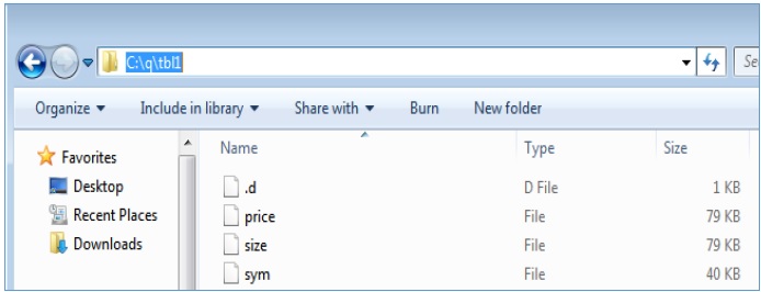
Partitioned Tables
Partitioned tables provide an efficient means to manage huge tables containing significant volumes of data. Partitioned tables are splayed tables spread across more partitions (directories).
Inside each partition, a table will have its own directory, with the structure of a splayed table. The tables could be split on a day/month/year basis in order to provide optimized access to its content.
To get the content of a partitioned table, use the following code block −
q)get `:c:/q/data/2000.01.13              // “get” command used, sample folder

quote| +`sym`time`bid`ask`bsize`asize`ex!(`p#`sym!0 0 0 0 0 0 0 0 0 0 0
0 0 0….

trade| +`sym`time`price`size`ex!(`p#`sym!0 0 0 0 0 0 0 0 0 0 0 0 0 0 0 0
0 0 ….
Let’s try to get the contents of a trade table −
q)get `:c:/q/data/2000.01.13/trade

   sym    time            price     size    ex
--------------------------------------------------
    0   09:30:00.496    0.4092016    7      T
    0   09:30:00.501    1.428629     4      N
    0   09:30:00.707    0.5647834    6      T
    0   09:30:00.781    1.590509     5      T
    0   09:30:00.848    2.242627     3      A
    0   09:30:00.860    2.277041     8      T
    0   09:30:00.931    0.8044885    8      A
    0   09:30:01.197    1.344031     2      A
    0   09:30:01.337    1.875        3      A
    0   09:30:01.399    2.187723     7      A
Note − The partitioned mode is suitable for tables with millions of records per day (i.e. time series data)
Sym file
The sym file is a kdb+ binary file containing the list of symbols from all splayed and partitioned tables. It can be read with,
get `:sym
par.txt file (optional)
This is a configuration file, used when partitions are spread on several directories/disk drives, and contain the paths to the disk partitions.
Q Language - Maintenance Functions
.Q.en
.Q.en is a dyadic function which help in splaying a table by enumerating a symbol column. It is especially useful when we are dealing with historical db (splayed, partition tables etc.). −
.Q.en[`:directory;table]
where directory is the home directory of the historical database where sym file is located and table is the table to be enumerated.
Manual enumeration of tables is not required to save them as splayed tables, as this will be done by −
.Q.en[`:directory_where_symbol_file_stored]table_name
.Q.dpft
The .Q.dpft function helps in creating partitioned and segmented tables. It is advanced form of .Q.en, as it not only splays the table but also creates a partition table.
There are four arguments used in .Q.dpft −
symbolic file handle of the database where we want to create a partition,
q data value with which we are going to partition the table,
name of the field with which parted (`p#) attribute is going to be applied (usually `sym), and
the table name.
Let’s take an example to see how it works −
q)tab:([]sym:5?`msft`hsbc`samsung`ibm;time:5?(09:30:30);price:5?30.25)

q).Q.dpft[`:c:/q/;2014.08.24;`sym;`tab]
`tab

q)delete tab from `
'type

q)delete tab from `/
'type

q)delete tab from .
'type

q)delete tab from `.
`.

q)tab
'tab
We have deleted the table tab from the memory. Let us now load it from the db
q)\l c:/q/2014.08.24/

q)\a
,`tab

q)tab

   sym      time      price
-------------------------------
  hsbc    07:38:13   15.64201
  hsbc    07:21:05   5.387037
  msft    06:16:58   11.88076
  msft    08:09:26   12.30159
 samsung  04:57:56   15.60838
.Q.chk
.Q.chk is a monadic function whose single parameter is the symbolic file handle of the root directory. It creates empty tables in a partition, wherever necessary, by examining each partition subdirectories in the root.
.Q.chk `:directory
where directory is the home directory of the historical database.