- Jupyter Tutorial
- Jupyter - Home
- IPython
- IPython - Introduction
- IPython - Installation
- IPython - Getting Started
- Running & Editing Python Script
- IPython - History Command
- IPython - System Commands
- IPython - Command Line Options
- Dynamic Object Introspection
- IPython - IO Caching
- Setting IPython as Default Python Environment
- Importing Python Shell Code
- IPython - Embedding IPython
- IPython - Magic Commands
- Jupyter
- Project Jupyter - Overview
- Jupyter Notebook - Introduction
- Working With Jupyter Online
- Installation and Getting Started
- Jupyter Notebook - Dashboard
- Jupyter Notebook - User Interface
- Jupyter Notebook - Types of Cells
- Jupyter Notebook - Editing
- Jupyter Notebook - Markdown Cells
- Cell Magic Functions
- Jupyter Notebook - Plotting
- Converting Notebooks
- Jupyter Notebook - IPyWidgets
- QtConsole
- QtConsole - Getting Started
- QtConsole - Multiline Editing
- QtConsole - Inline Graphics
- QtConsole - Save to Html
- QtConsole - Multiple Consoles
- Connecting to Jupyter Notebook
- Using github and nbviewer
- JupyterLab
- JupyterLab - Overview
- Installation & Getting Started
- JupyterLab - Interface
- JupyterLab - Installing R Kernel
- Jupyter Resources
- Jupyter - Quick Guide
- Jupyter - Useful Resources
- Jupyter - Discussion
Jupyter - Quick Guide
IPython - Introduction
Project Jupyter is a suite of software products used in interactive computing. IPython was originally developed by Fernando Perez in 2001 as an enhanced Python interpreter. A web based interface to IPython terminal in the form of IPython notebook was introduced in 2011. In 2014, Project Jupyter started as a spin-off project from IPython.
Packages under Jupyter project include −
Jupyter notebook − A web based interface to programming environments of Python, Julia, R and many others
QtConsole − Qt based terminal for Jupyter kernels similar to IPython
nbviewer − Facility to share Jupyter notebooks
JupyterLab − Modern web based integrated interface for all products.
Standard distribution of Python comes with a REPL (Read-Evaluate-Print Loop) environment in the form of Python shell with >>> prompt. IPython (stands for Interactive Python) is an enhanced interactive environment for Python with many functionalities compared to the standard Python shell.
Features of IPython
IPython offers more features compared to the standard Python. They are as follows −
Offers a powerful interactive Python shell.
Acts as a main kernel for Jupyter notebook and other front end tools of Project Jupyter.
Possesses object introspection ability. Introspection is the ability to check properties of an object during runtime.
Syntax highlighting.
Stores the history of interactions.
Tab completion of keywords, variables and function names.
Magic command system useful for controlling Python environment and performing OS tasks.
Ability to be embedded in other Python programs.
Provides access to Python debugger.
History and Development
IPython was originally developed by Fernando Perez in 2001. Its current version is IPython7.0.1 which requires Python 3.4 version or higher. IPython 6.0 was the first version to support Python 3. Users having Python 2.7 should work with IPython’s version 2.0 to 5.7
The concept of computational notebooks started in 80s decade when MATLAB and Mathematica were released. These GUI frontends to the interactive shell had features like text formatting, adding graphics, table and adding mathematical symbols. Sage notebook is also a web based notebook.
Creaters of IPython started working on notebook interface for IPython shell in 2005. IPython notebook soon added support of other languages like R and Julia. It was in 2014, that Perez started Jupyter project as a spin-off project from IPython, since IPython project was becoming big with products like notebook server and Qt console added to it.
Since IPython 4.0, all additional components were shifted to Project Jupyter and adding support of other languages to IPython notebook. IPython continues to focus on improvement of its enhanced interpreter feature. It also provides primary kernel to Jupyter notebook frontend.
IPython - Installation
IPython is included by default in Anaconda distribution of Python. It can be downloaded from Anaconda’s download page www.anaconda.com/download/ Binaries for all major OS (Windows, MacOS and Linux) and architecture (32 bit and 64 bit) are available on this link.
To install IPython separately in standard Python installation, you can use pip command as shown below −
pip3 install ipython
IPython internally uses following packages −
| Sr.No. | IPython dependencies & Functionality |
|---|---|
| 1 | colorama Cross-platform API for printing colored terminal text from Python |
| 2 | jedi An autocompletion tool for Python |
| 3 | pickleshare Small ‘shelve’ like datastore with concurrency support |
| 4 | prompt_toolkit Library for building powerful interactive command lines in Python |
| 5 | pygments Syntax highlighting package written in Python |
| 6 | simplegeneric Simple generic functions |
| 7 | traitlets Configuration system for Python applications. |
In general, all dependencies get installed automatically. Else, you can install them individually using pip.
IPython - Getting Started
This chapter will explain how to get started with working on IPython.
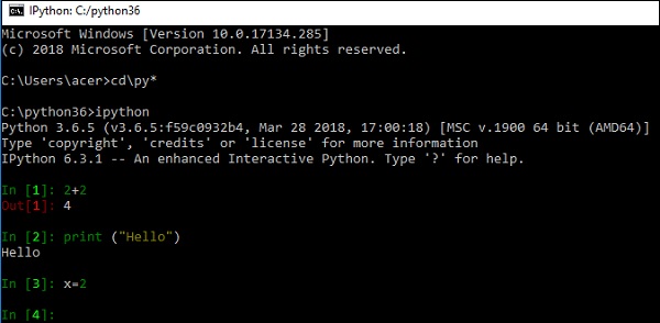
Starting IPython from Command Prompt.
Before proceeding to understand about IPython in depth, note that instead of the regular >>>, you will notice two major Python prompts as explained below −
In[1] appears before any input expression.
Out[1] appears before the Output appears.
Besides, the numbers in the square brackets are incremented automatically. Observe the following screenshot for a better understanding −
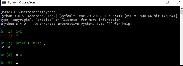
Now, if you have installed Anaconda distribution of Python, open Anaconda prompt from start menu.
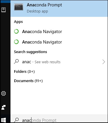
Start IPython from conda prompt
When compared to regular Python console, we can notice a difference. The IPython shell shows syntax highlighting by using different colour scheme for different elements like expression, function, variable etc.
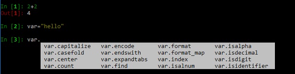
Another useful enhancement is tab completion. We know that each object has one or more methods available as defined in its class. IPython pops up appropriate list of methods as you press tab key after dot in front of object.
In the following example, a string is defined. As a response, the methods of string class are shown.
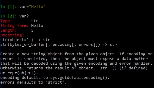
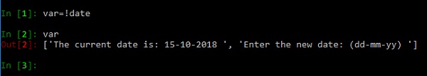
IPython provides information of any object by putting ‘?’ in front of it. It includes docstring, function definitions and constructor details of class. For example to explore the string object var defined above, in the input prompt enter var?. The result will show all information about it. Observe the screenshot given below for a better understanding −
Magic Functions
IPython’s in-built magic functions are extremely powerful. There are two types of magic functions.
- Line magics, which work very much like DOS commands.
- Cell magics, which work on multiple lines of code.
We shall learn about line magic functions and cell magic functions in detail in subsequent chapters.
IPython - Running and Editing Python Script
In this chapter, let us understand how to run and edit a Python script.
Run Command
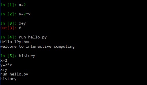
You can use run command in the input prompt to run a Python script. The run command is actually line magic command and should actually be written as %run. However, the %automagic mode is always on by default, so you can omit this.
In [1]: run hello.py
Hello IPython
Edit Command
IPython also provides edit magic command. It invokes default editor of the operating system. You can open it through Windows Notepad editor and the script can be edited. Once you close it after saving its input, the output of modified script will be displayed.
In [2]: edit hello.py
Editing... done. Executing edited code...
Hello IPython
welcome to interactive computing
Note that hello.py initially contained only one statement and after editing one more statement was added. If no file name is given to edit command, a temporary file is created. Observe the following code that shows the same.
In [7]: edit
IPython will make a temporary file named:
C:\Users\acer\AppData\Local\Temp\ipython_edit_4aa4vx8f\ipython_edit_t7i6s_er.py
Editing... done. Executing edited code...
magic of IPython
Out[7]: 'print ("magic of IPython")'
IPython - History Command
IPython preserves both the commands and their results of the current session. We can scroll through the previous commands by pressing the up and down keys.
Besides, last three objects of output are stored in special variables _, __ and ___. The history magic command shows previous commands in current session as shown in the screenshot given below −
IPython - System Commands
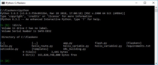
If the statement in the input cell starts with the exclamation symbol (!), it is treated as a system command for underlying operating system. For example, !ls (for linux) and !dir (for windows) displays the contents of current directory
The output of system command can also be assigned to a Python variable as shown below −
The variable stores output without colors and splits at newline characters.
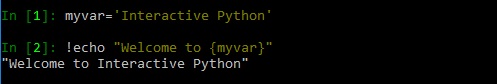
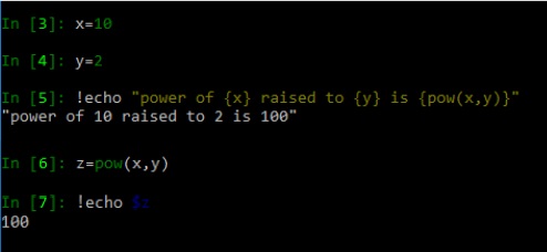
It is also possible to combine Python variables or expressions with system command calls. Variable in curly brackets {} can be embedded in command text. Observe the following example −
Here is another example to understand that prefixing Python variable with $ also achieves the same result.
IPython - Command Line Options
In this chapter, let us understand how to work with various command line options in IPython.
Invoking IPython Program
You can invoke an IPython program using the following options −
C:\python36> ipython [subcommand] [options] [-c cmd | -m mod | file] [--] [arg]
The file option is a Python script with .py extension. If no other option is given, the script is executed and command prompt reappears.
C:\python36>ipython hello.py
Hello IPython
welcome to interactive computing
Subcommands and Parameters
An IPython command accepts the following subcommand options −
Profile − Create and manage IPython profiles.
Kernel − Start a kernel without an attached frontend.
Locate − Print the path to the IPython dir.
History − Manage the IPython history database.
An IPython profile subcommand accepts the following parameters −
ipython profile create myprofile − Creates a new profile.
ipython profile list − Lists all available profiles.
ipython locate profile myprofile − Locates required profile.
To install new IPython kernel, use the following command −
Ipython kernel –install –name
To print the path to the IPython dir, use the following command −
C:\python36>ipython locate myprofile
C:\Users\acer\.ipython
Besides, we know that −
The history subcommand manages IPython history database.
The trim option reduces the IPython history database to the last 1000 entries.
The clear option deletes all entries.
Some of the other important command line options of IPython are listed below −
| Sr.No. | IPython Command & Description |
|---|---|
| 1 | --automagic Turn on the auto calling of magic commands. |
| 2 | --pdb Enable auto calling the pdb debugger after every exception. |
| 3 | --pylab Pre-load matplotlib and numpy for interactive use with the default matplotlib backend. |
| 4 | --matplotlib Configure matplotlib for interactive use with the default matplotlib backend. |
| 5 | --gui=options Enable GUI event loop integration with any of ('glut', 'gtk', 'gtk2','gtk3', 'osx', 'pyglet', 'qt', 'qt4', 'qt5', 'tk', 'wx', 'gtk2', 'qt4'). |
The sample usage of some of the IPython command line options are shown in following table −
| Sr.No. | IPython Command & Description |
|---|---|
| 1 | ipython --matplotlib enable matplotlib integration |
| 2 | ipython --matplotlib=qt enable matplotlib integration with qt4 backend |
| 3 | ipython --profile=myprofile start with profile foo |
| 4 | ipython profile create myprofile create profile foo w/ default config files |
| 5 | ipython help profile show the help for the profile subcmd |
| 6 | ipython locate print the path to the IPython directory |
| 7 | ipython locate profile myprofile print the path to the directory for profile `myprofile` |
IPython - Dynamic Object Introspection
IPython has different ways of obtaining information about Python objects dynamically. In this chapter, let us learn the ways of dynamic object introspection in IPython.
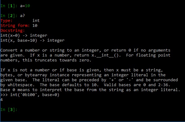
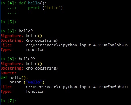
Use of ? and ?? provides specific and more detailed information about the object. In the first example discussed below, a simple integer object a is created. Its information can be procured by typing a ? in the input cell.
In the second example, let us define a function and introspect this function object with ? and ??.
Note that the magic function %psearch is equivalent to the use of ? or ?? for fetching object information.
IPython - IO Caching
The input and output cells on IPython console are numbered incrementally. In this chapter, let us look into IO caching in Python in detail.
In IPython, inputs are retrieved using up arrow key. Besides, all previous inputs are saved and can be retrieved. The variables _i, __i, and ___i always store the previous three input entries. In addition, In and _in variables provides lists of all inputs. Obviously _in[n] retrieves input from nth input cell. The following IPython session helps you to understand this phenomenon −
In [1]: print ("Hello")
Hello

In [2]: 2+2
Out[2]: 4

In [3]: x = 10

In [4]: y = 2

In [5]: pow(x,y)
Out[5]: 100

In [6]: _iii, _ii, _i
Out[6]: ('x = 10', 'y = 2', 'pow(x,y)')

In [7]: In
Out[7]:
['',
   'print ("Hello")',
   '2+2',
   'x = 10',
   'y = 2',
   'pow(x,y)',
   '_iii, _ii, _i',
   'In'
]

In [8]: In[5] 9. IPython — IO
Out[8]: 'pow(x,y)'

In [9]: _ih
Out[9]:
['',
   'print ("Hello")',
   '2+2',
   'x = 10',
   'y = 2',
   'pow(x,y)',
   '_iii, _ii, _i',
   'In',
   'In[5]',
   '_ih'
]

In [11]: _ih[4]
Out[11]: 'y = 2'

In [12]: In[1:4]
Out[12]: ['print ("Hello")', '2+2', 'x=10']
Similarly, single, double and triple underscores act as variables to store previous three outputs. Also Out and _oh form a dictionary object of cell number and output of cells performing action (not including assignment statements). To retrieve contents of specific output cell, use Out[n] or _oh[n]. You can also use slicing to get output cells within a range.
In [1]: print ("Hello")
Hello

In [2]: 2+2
Out[2]: 4

In [3]: x = 10

In [4]: y = 3

In [5]: pow(x,y)
Out[5]: 1000

In [6]: ___, __, _
Out[6]: ('', 4, 1000)

In [7]: Out
Out[7]: {2: 4, 5: 1000, 6: ('', 4, 1000)}

In [8]: _oh
Out[8]: {2: 4, 5: 1000, 6: ('', 4, 1000)}

In [9]: _5
Out[9]: 1000

In [10]: Out[6]
Out[10]: ('', 4, 1000)
Setting IPython as Default Python Environment
Different environment variables influence Python’s behaviour. PYTHONSTARTUP environment variable is assigned to a Python script. As an effect, this script gets executed before Python prompt appears. This is useful if certain modules are to be loaded by default every time a new Python session starts.
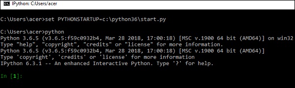
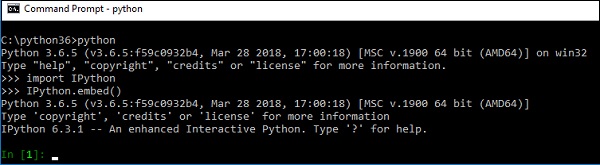
The following script (start.py) imports IPython module and executes start_ipython() function to replace default Python shell with prompt (>>>) by IPython shell when Python executable is invoked.
import os, IPython
os.environ['PYTHONSTARTUP'] = ''
IPython.start_ipython()
raise SystemExit
Assuming that this file is stored in Python’s installation directory (c:\python36), set PYTHONSTARTUP environment variable and start Python from command line. Then IPython shell appears as shown below −
Note that the environment variable can be permanently set using System Properties dialog in Windows and using export command on Linux.
IPython - Importing Python Shell Code
IPython can read from standard Python console with default >>> prompt and another IPython session. The following screenshot shows a for loop written in standard Python shell −
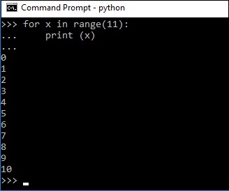
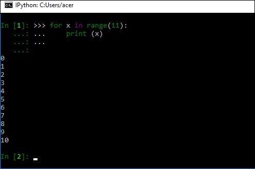
Copy the code (along with Python prompt) and paste the same in IPython input cell. IPython intelligently filters out the input prompts (>>> and ...) or IPython ones (In [N]: and ...:)
Similarly, code from one IPython session can be pasted in another. The first screenshot given below shows definition of SayHello() function in one IPython window −
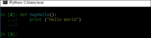
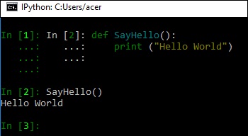
Now, let us select the code and paste in another IPython shell and call SayHello() function.
Embedding IPython
The embed() function of IPython module makes it possible to embed IPython in your Python codes’ namespace. Thereby you can leverage IPython features like object introspection and tab completion, in default Python environment.
Python objects present in the global namespace before embedding, will be available to IPython.
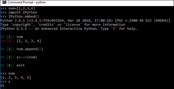
If new objects are formed while in IPython or previous objects are modified, they will be automatically available to default environment after exiting IPython. Embedded IPython shell doesn’t change the state of earlier code or objects.
However, if IPython is embedded in local namespace like inside a function, the objects inside it will not be available once it is closed. Here, we have defined a function add(). Inside add() we invoke IPython and declared a variable. If we try to access variable in IPython after it is closed, NameError exception will be raised.

IPython - Magic Commands
Magic commands or magic functions are one of the important enhancements that IPython offers compared to the standard Python shell. These magic commands are intended to solve common problems in data analysis using Python. In fact, they control the behaviour of IPython itself.
Magic commands act as convenient functions where Python syntax is not the most natural one. They are useful to embed invalid python syntax in their work flow.
Types of Magic Commands
There are two types of magic commands −
- Line magics
- Cell magics
Line Magics
They are similar to command line calls. They start with % character. Rest of the line is its argument passed without parentheses or quotes. Line magics can be used as expression and their return value can be assigned to variable.
Cell Magics
They have %% character prefix. Unlike line magic functions, they can operate on multiple lines below their call. They can in fact make arbitrary modifications to the input they receive, which need not even be a valid Python code at all. They receive the whole block as a single string.
To know more about magic functions, the built-in magics and their docstrings, use the magic command. Information of a specific magic function is obtained by %magicfunction? Command. Let us now describe some of the built-in line and cell magic commands.
Built-in line magics
%autocall [mode]
This magic function makes a function automatically callable without having to use parentheses. It takes three possible mode parameters: 0 (off), 1 (smart) is default or 2 (always on).
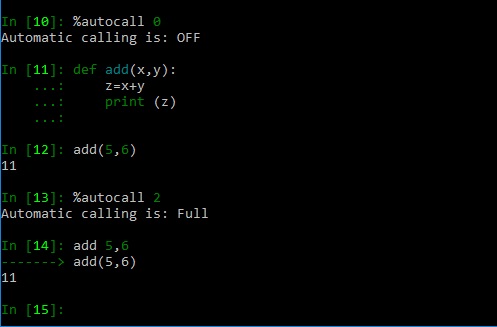
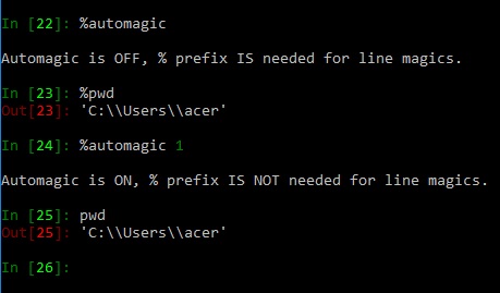
%automagic
Magic functions are callable without having to type the initial % if set to 1. Without arguments it toggles on/off. To deactivate, set to 0.
The following example shows a magic function %pwd (displays present working directory) being called without leading % when %automagic set to 1
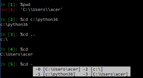
%cd
This line magic changes the current directory. This command automatically maintains an internal list of directories you visit during your IPython session, in the variable _dh. You can also do ‘cd -<tab>’ to see directory history conveniently.
Usage
The %cd command can be used in the following ways −
%cd <dir> − Changes current working directory to <dir>
%cd.. − Changes current directory to parent directory
%cd − changes to last visited directory.
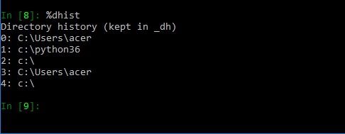
%dhist
This magic command prints all directories you have visited in current session. Every time %cd command is used, this list is updated in _dh variable.
%edit
This magic command calls upon the default text editor of current operating system (Notepad for Windows) for editing a Python script. The script is executed as the editor is closed.
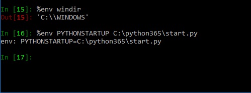
%env
This magic command will list all environment variables. It also reads value of particular variable or set the value of environment variable.
Usage
The %cd command can be used in the following ways −
%env − Lists all environment variables
%env var − Gets value for var
%env var val − Sets value for var
%gui [GUINAME]
When used without argument this command enables or disables IPython GUI event loop integration. With GUINAME argument, this magic replaces the default GUI toolkits by the specified one.
| Sr.No. | Command & Description |
|---|---|
| 1 | %gui wx enable wxPython event loop integration |
| 2 | %gui qt4|qt enable PyQt4 event loop integration |
| 3 | %gui qt5 enable PyQt5 event loop integration |
| 4 | %gui gtk enable PyGTK event loop integration |
| 5 | %gui gtk3 enable Gtk3 event loop integration |
| 6 | %gui tk enable Tk event loop integration |
| 7 | %gui osx enable Cocoa event loop integration |
| 8 | (requires %matplotlib 1.1) |
| 9 | %gui disable all event loop integration |
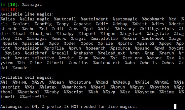
%lsmagic
Displays all magic functions currently available
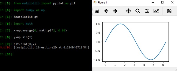
%matplotlib
This function activates matplotlib interactive support during an IPython session. However, it does not import matplotlib library. The matplotlib default GUI toolkit is TkAgg. But you can explicitly request a different GUI backend. You can see a list of the available backends as shown −
In [4]: %matplotlib --list
Available matplotlib backends:
['osx', 'qt4', 'qt5', 'gtk3', 'notebook', 'wx', 'qt', 'nbagg','gtk', 'tk', 'inline']
The IPython session shown here plots a sine wave using qt toolkit −
While using Jupyter notebook, %matplotlib inline directive displays plot output in the browser only.
%notebook
This function converts current IPython history into an IPython notebook file with ipynb extension. The input cells in previous example are saved as sine.ipynb
%notebook sine.ipynb
%pinfo
This function is similar to object introspection ? character. To obtain information about an object, use the following command −
%pinfo object
This is synonymous to object? or ?object.
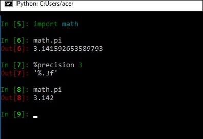
%precision
This magic function restricts a floating point result to specified digits after decimal.
%pwd
This magic function returns the present working directory.

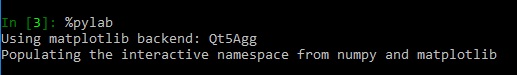
%pylab
This function populates current IPython session with matplotlib, and numpy libraries.
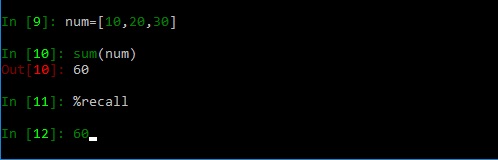
%recall
When executed without any parameter, this function executes previous command.
Note that in %recall n, number in front of it is input cell number. Hence the command in the nth cell is recalled. You can recall commands in section of cells by using command such as %recall 1-4. Current input cell is populated with recalled cell and the cursor blinks till the enter key is pressed.
%run
This command runs a Python script from within IPython shell.

%time
This command displays time required by IPython environment to execute a Python expression.

%timeit
This function also displays time required by IPython environment to execute a Python expression. Time execution of a Python statement or expression uses the timeit module. This function can be used both as a line and cell magic as explained here −
In line mode you can time a single-line.
In cell mode, the statement in the first line is used as setup code and the body of the cell is timed. The cell body has access to any variables created in the setup code.
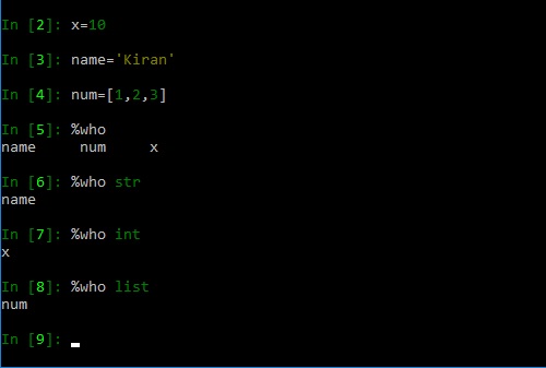
%who
This line magic prints all interactive variables, with some minimal formatting. If any arguments are given, only variables whose type matches one of these are printed.
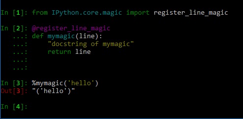
IPython Custom Line Magic function
IPython’s core library contains register_line_magic decorator. A user defined function is converted into a line magic function using this decorator.
Project Jupyter - Overview
Project Jupyter started as a spin-off from IPython project in 2014. IPython’s language-agnostic features were moved under the name – Jupyter. The name is a reference to core programming languages supported by Jupyter which are Julia, Python and RProducts under Jupyter project are intended to support interactive data science and scientific computing.
The project Jupyter consists of various products described as under −
IPykernel − This is a package that provides IPython kernel to Jupyter.
Jupyter client − This package contains the reference implementation of the Jupyter protocol. It is also a client library for starting, managing and communicating with Jupyter kernels.
Jupyter notebook − This was earlier known as IPython notebook. This is a web based interface to IPython kernel and kernels of many other programming languages.
Jupyter kernels − Kernel is the execution environment of a programming language for Jupyter products.
The list of Jupyter kernels is given below −
| Kernel | Language | URL |
|---|---|---|
| IJulia | Julia | |
| IHaskell | Haskell | |
| IRuby | Ruby | |
| IJavaScript | JavaScript | |
| IPHP | PHP | |
| IRKernel | R |
Qtconsole − A rich Qt-based console for working with Jupyter kernels
nbconvert − Converts Jupyter notebook files in other formats
JupyterLab − Web based integrated interface for notebooks, editors, consoles etc.
nbviewer − HTML viewer for notebook files
Jupyter Notebook - Introduction
IPython notebook was developed by Fernando Perez as a web based front end to IPython kernel. As an effort to make an integrated interactive computing environment for multiple language, Notebook project was shifted under Project Jupyter providing front end for programming environments Juila and R in addition to Python.
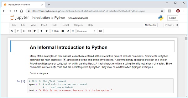
A notebook document consists of rich text elements with HTML formatted text, figures, mathematical equations etc. The notebook is also an executable document consisting of code blocks in Python or other supporting languages.
Jupyter notebook is a client-server application. The application starts the server on local machine and opens the notebook interface in web browser where it can be edited and run from. The notebook is saved as ipynb file and can be exported as html, pdf and LaTex files.
Working with Jupyter Online
If you are new to Jupyter, you can try features of Jupyter notebook before installing on your local machine. For this purpose, visit https://jupyter.org in your browser and choose ‘Try Jupyter with Python’ option.
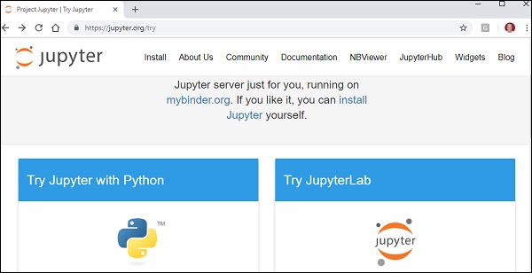
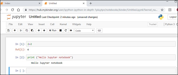
This will open home page of https://mybinder.org From the File menu, choose new notebook option to open a blank Jupyter in your browser. The input cell, as similar to that in IPython terminal, will be displayed. You can execute any Python expression in it.
Installation and Getting Started
You can easily install Jupyter notebook application using pip package manager.
pip3 install jupyter
To start the application, use the following command in the command prompt window.
c:\python36>jupyter notebook
The server application starts running at default port number 8888 and browser window opens to show notebook dashboard.
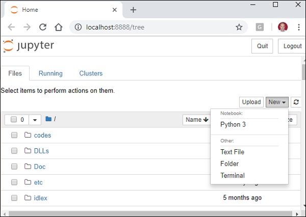
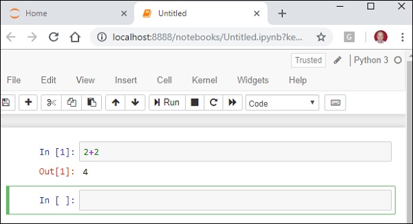
Observe that the dashboard shows a dropdown near the right border of browser with an arrow beside the New button. It contains the currently available notebook kernels. Now, choose Python 3, then a new notebook opens in a new tab. An input cell as similar to that of in IPython console is displayed.
You can execute any Python expression in it. The result will be displayed in the Out cell.
Jupyter Notebook - Dashboard
The dashboard of Jupyter Notebook contains three tabs as shown in the screenshot given below −
Files Tab
The "Files" tab displays files and folders under current directory from which notebook app was invoked. The row corresponding to a notebook which is currently open and the running status is shown just beside the last modified column. It also displays Upload button using which a file can be uploaded to notebook server.
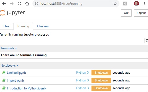
Running Tab
The "Running" tab shows which of the notebooks are currently running.
Cluster Tab
The third tab, "Clusters", is provided by IPython parallel. IPython's parallel computing framework, an extended version of the IPython kernel.
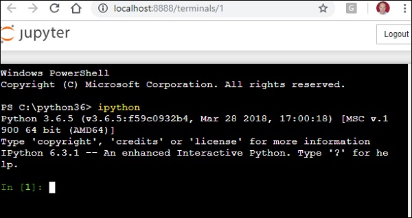
From the New dropdown choose Terminal to open a cmd window. You can now start an IPython terminal here.
Jupyter Notebook - User Interface
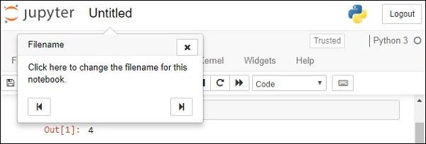
In the user interface of Jupyter, just beside the logo in the header, the file name is displayed.
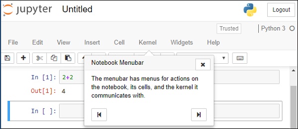
You can find the menu bar below the header. Each menu contains many options that will be discussed later.
A row of icons forming toolbar helps user to perform often required operations
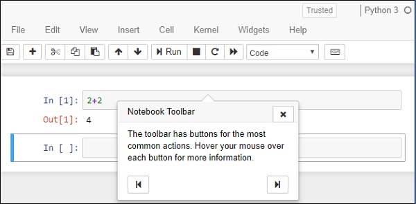
The notebook has two modes − Command mode and Edit mode. Notebook enters edit mode when a cell is clicked. Notice the pencil symbol just besides name of kernel.

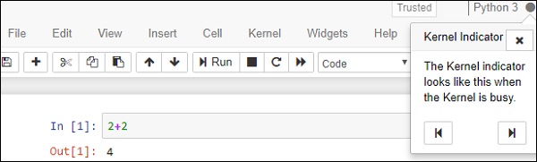
Kernel indicator symbol is displayed just to the right of kernel name. Note that a hollow circle means kernel is idle and solid circle means it is busy.
File Menu
The following are the options available in the File menu −
| Sr.No. | File menu & Description |
|---|---|
| 1 | New notebook choose the kernel to start new notebook |
| 2 | Open Takes user to dashboard to choose notebook to open |
| 3 | Save as save current notebook and start new kernel |
| 4 | Rename rename current notebook |
| 5 | Save saves current notebook and stores current checkpoint |
| 6 | Revert reverts state of notebook to earlier checkpoint |
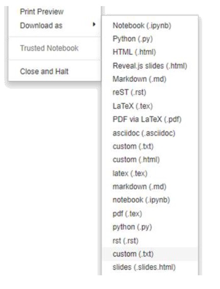
| 7 | Download export notebook in one of various file formats |
The file formats that are available are shown below −
Edit Menu
Edit menu consists of buttons to perform cut, copy and paste cells, delete selected cell, split and merge cells, move cells up and down, find and replace within notebook, cut/copy attachments and insert image.
View Menu
Buttons in this menu help us to hide/display header, toolbar and cell numbers.
Insert Menu
This menu gives you options for inserting cell before or after the current cell.
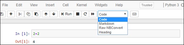
Cell Menu
The options in this menu let user run all or specific cells in the notebook. You can also set the cell type to code type, markdown or raw nbconvert type.
Kernel Menu
From this menu you can start, interrupt, restart or shutdown the kernel. You can also start a new kernel.
Widgets Menu
From this menu you can save, clear, download or embed widget state.
Help menu
Various predefined keyboard shortcuts are displayed from this menu. You can also edit the shortcuts as per your convenience.
Jupyter Notebook - Types of Cells
Cells in Jupyter notebook are of three types − Code, Markdown and Raw.
Code Cells
Contents in this cell are treated as statements in a programming language of current kernel. Default kernel is Python. So, we can write Python statements in a code cell. When such cell is run, its result is displayed in an output cell. The output may be text, image, matplotlib plots or HTML tables. Code cells have rich text capability.
Markdown Cells
These cells contain text formatted using markdown language. All kinds of formatting features are available like making text bold and italic, displaying ordered or unordered list, rendering tabular contents etc. Markdown cells are especially useful to provide documentation to the computational process of the notebook.
Raw Cells
Contents in raw cells are not evaluated by notebook kernel. When passed through nbconvert, they will be rendered as desired. If you type LatEx in a raw cell, rendering will happen after nbconvert is applied.
Jupyter Notebook - Editing
While the menu bar and toolbar lets you perform various operations on notebook, it is desirable to be able to use keyboard shortcuts to perform them quickly.
Jupyter Notebooks have two different keyboard input modes −
Command Mode − Binds the keyboard to notebook level actions. Indicated by a grey cell border with a blue left margin.
Edit Mode − When you are typing in a cell. Indicated by a green cell border.
Command Mode (press Esc to enable)
F |
find and replace | 1 |
change cell to heading 1 |
Ctrl-Shift-F |
open the command palette | 2 |
change cell to heading 2 |
Ctrl-Shift-P |
open the command palette | 3 |
change cell to heading 3 |
Enter |
enter edit mode | 4 |
change cell to heading 4 |
P |
open the command palette | 5 |
change cell to heading 5 |
Shift-Enter |
run cell, select below | 6 |
change cell to heading 6 |
Ctrl-Enter |
run selected cells | A |
insert cell above |
Alt-Enter |
run cell and insert below | B |
insert cell below |
Y |
change cell to code | X |
cut selected cells |
M |
change cell to markdown | C |
copy selected cells |
R |
change cell to raw | V |
paste cells below |
K |
select cell above | Z |
undo cell deletion |
Up |
select cell above | D,D |
delete selected cells |
Down |
select cell below | Shift-M |
merge selected cells, or current cell with cell below if only one cell is selected |
J |
select cell below | Shift-V |
paste cells above |
Shift-K |
extend selected cells above | L |
toggle line numbers |
Shift-Up |
extend selected cells above | O |
toggle output of selected cells |
Shift-Down |
extend selected cells below | Shift-O |
toggle output scrolling of selected cells |
Shift-J |
extend selected cells below | I,I |
interrupt the kernel |
Ctrl-S |
Save and Checkpoint | 0,0 |
restart the kernel (with dialog) |
S |
Save and Checkpoint | Esc |
close the pager |
Shift-L |
toggles line numbers in all cells, and persist the setting | Q |
close the pager |
Shift-Space |
scroll notebook up | Space |
scroll notebook down |
Edit Mode (press Enter to enable)
Tab |
code completion or indent | Ctrl-Home |
go to cell start |
Shift-Tab |
tooltip | Ctrl-Up |
go to cell start |
Ctrl-] |
indent | Ctrl-End |
go to cell end |
Ctrl-[ |
dedent | Ctrl-Down |
go to cell end |
Ctrl-A |
select all | Ctrl-Left |
go one word left |
Ctrl-Z |
undo | Ctrl-Right |
go one word right |
Ctrl-/ |
comment | Ctrl-M |
enter command mode |
Ctrl-D |
delete whole line | Ctrl-Shift-F |
open the command palette |
Ctrl-U |
undo selection | Ctrl-Shift-P |
open the command palette |
Insert |
toggle overwrite flag | Esc |
enter command mode |
Ctrl-Backspace |
delete word before | Ctrl-Y |
redo |
Ctrl-Delete |
delete word after | Alt-U |
redo selection |
Shift-Enter |
run cell, select below | Ctrl-Shift-Minus |
split cell at cursor |
Ctrl-Enter |
run selected cells | Down |
move cursor down |
Alt-Enter |
run cell and insert below | Up |
move cursor up |
Ctrl-S |
Save and Checkpoint |
Jupyter Notebook - Markdown Cells
Markdown cell displays text which can be formatted using markdown language. In order to enter a text which should not be treated as code by Notebook server, it must be first converted as markdown cell either from cell menu or by using keyboard shortcut M while in command mode. The In[] prompt before cell disappears.
Header cell
A markdown cell can display header text of 6 sizes, similar to HTML headers. Start the text in markdown cell by # symbol. Use as many # symbols corresponding to level of header you want. It means single # will render biggest header line, and six # symbols renders header of smallest font size. The rendering will take place when you run the cell either from cell menu or run button of toolbar.
Following screenshot shows markdown cells in edit mode with headers of three different levels.
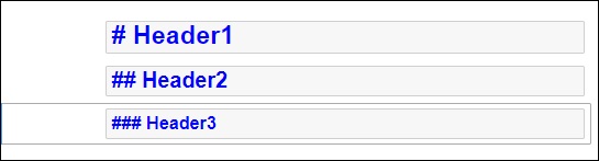
When cells are run, the output is as follows −

Note that Jupyter notebook markdown doesn’t support WYSWYG feature. The effect of formatting will be rendered only after the markdown cell is run.
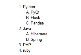
Ordered Lists
To render a numbered list as is done by <ol> tag of HTML, the First item in the list should be numbered as 1. Subsequent items may be given any number. It will be rendered serially when the markdown cell is run. To show an indented list, press tab key and start first item in each sublist with 1.
If you give the following data for markdown −
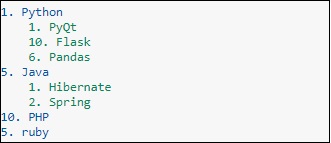
It will display the following list −
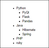
Bullet lists
Each item in the list will display a solid circle if it starts with – symbol where as solid square symbol will be displayed if list starts with * symbol. The following example explains this feature −
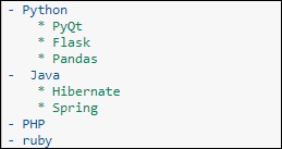
The rendered markdown shows up as below −
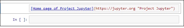
Hyperlinks
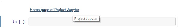
Markdown text starting with http or https automatically renders hyperlink. To attach link to text, place text in square brackets [] and link in parentheses () optionally including hovering text. Following screenshot will explain this.
The rendered markdown appears as shown below −
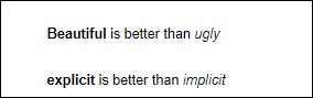
Bold and Italics
To show a text in bold face, put it in between double underscores or two asterisks. To show in italics, put it between single underscores or single asterisks.

The result is as shown below −
Images
To display image in a markdown cell, choose ‘Insert image’ option from Edit menu and browse to desired image file. The markdown cell shows its syntax as follows −
Image will be rendered on the notebook as shown below −
Table
In a markdown cell, a table can be constructed using | (pipe symbol) and – (dash) to mark columns and rows. Note that the symbols need not be exactly aligned while typing. It should only take respective place of column borders and row border. Notebook will automatically resize according to content. A table is constructed as shown below −
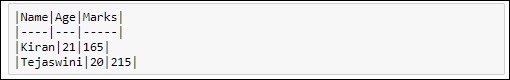
The output table will be rendered as shown below −

Jupyter Notebook - Cell Magic Functions
In this chapter, let us understand cell magic functions and their functionalities.
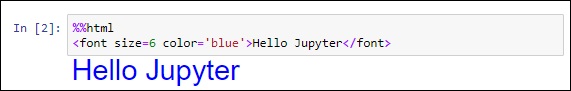
%%html
This cell magic function renders contents of code cell as html script.
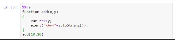
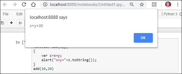
%%js or %%javascript
You can embed javascript code in Jupyter notebook cell with the help of this cell magic command.
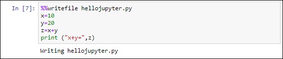
%%writefile
Contents of code cell are written to a file using this command.
Jupyter Notebook - Plotting
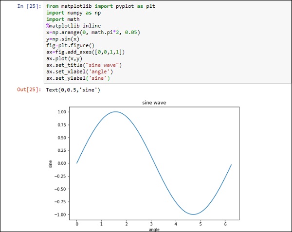
IPython kernel of Jupyter notebook is able to display plots of code in input cells. It works seamlessly with matplotlib library. The inline option with the %matplotlib magic function renders the plot out cell even if show() function of plot object is not called. The show() function causes the figure to be displayed below in[] cell without out[] with number.
Now, add plt.show() at the end and run the cell again to see the difference.
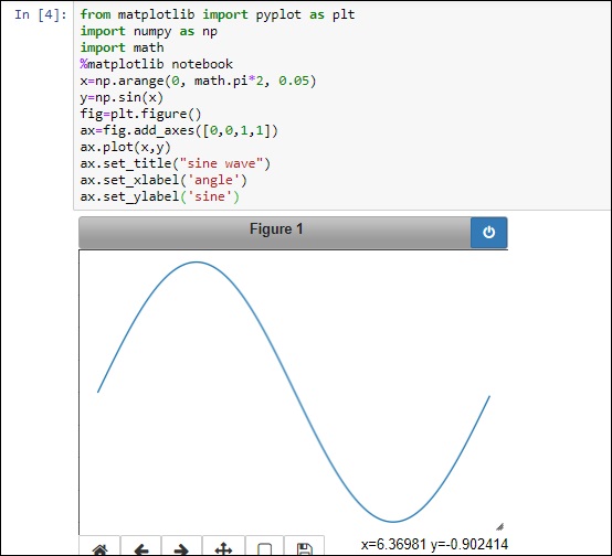
Note that the %matplotlib notebook magic renders interactive plot.
Just below the figure, you can find a tool bar to switch views, pan, zoom and download options.
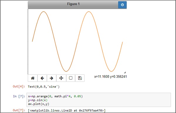
Importantly, if you modify the data underneath the plot, the display changes dynamically without drawing another plot.
In the above example, change the data sets of x and y in the cell below and plot the figure again, the figure above will get dynamically refreshed.
Jupyter - Converting Notebooks
Jupyter notebook files have .ipynb extension. Notebook is rendered in web browser by the notebook app. It can be exported to various file formats by using download as an option in the file menu. Jupyter also has a command line interface in the form of nbconvert option. By default, nbconvert exports the notebook to HTML format. You can use the following command for tis purpose −
jupyter nbconvert mynotebook.ipynb
This will convert mynotebook.ipynb to the mynotebook.html. Other export format is specified with `--to` clause.
Note that other options include ['asciidoc', 'custom', 'html', 'latex', 'markdown', 'notebook', 'pdf', 'python', 'rst', 'script', 'slides']
HTML includes 'basic' and 'full' templates. You can specify that in the command line as shown below −
jupyter nbconvert --to html --template basic mynotebook.ipynb
LaTex is a document preparation format used specially in scientific typesetting. Jupyter includes 'base', 'article' and 'report' templates.
jupyter nbconvert --to latex –template report mynotebook.ipynb
To generate PDF via latex, use the following command −
jupyter nbconvert mynotebook.ipynb --to pdf
Notebook can be exported to HTML slideshow. The conversion uses Reveal.js in the background. To serve the slides by an HTTP server, add --postserve on the command-line. To make slides that does not require an internet connection, just place the Reveal.js library in the same directory where your_talk.slides.html is located.
jupyter nbconvert myslides.ipynb --to slides --post serve
The markdown option converts notebook to simple markdown output. Markdown cells are unaffected, and code cells indented 4 spaces.
--to markdown
You can use rst option to convert notebook to Basic reStructuredText output. It is useful as a starting point for embedding notebooks in Sphinx docs.
--to rst
This is the simplest way to get a Python (or other language, depending on the kernel) script out of a notebook.
--to script
Jupyter Notebook - IPyWidgets
IPyWidgets is a Python library of HTML interactive widgets for Jupyter notebook. Each UI element in the library can respond to events and invokes specified event handler functions. They enhance the interactive feature of Jupyter notebook application.
In order to incorporate widgets in the notebook, we have to import the following module as shown below −
from ipywidgets import widgets
Some basic IPyWidgets are explained here −
Text input
The widgets.text() function renders widgets in the notebook. It is similar to text box form element in HTML. The object of this widget has on_submit() method which listens to activity of the text field and can invoke event handler given as an argument to it.
Button
This widget is similar to HTML button. When it is clicked, the event is registered by on_click() method which calls the click event handler.
IntSlider
A slider control which displays the incrementing integer values. There is also a FloatSlider and IntRangeSlider (changing integer between a range)
Label
This widget is useful to display non editable text in the notebook.
display()
This function from ipywidgets module renders the widget object in notebook’s input cell.
Interact
This function automatically renders a widget depending upon type of data argument given to it. First argument to this function is the event handler and second is a value passed to event handler itself.
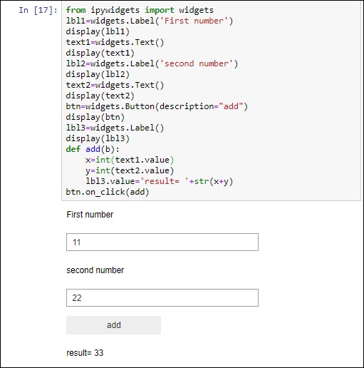
Following example shows three label widgets, two text widgets and a button with ‘add’ caption. When the button is clicked, sum of numbers in two text input fields is displayed on the lowermost label.
Jupyter QtConsole - Getting Started
In this chapter, let us understand how to get started with QtConsole. This chapter will give you an overview about this software and explains its installation steps.
Overview
The Qt console is a GUI application similar to IPython terminal. However, it provides a number of enhancements which are not available in text based IPython terminal. The enhance features are inline figures, multi-line editing with syntax highlighting, graphical calltips, etc. The Qt console can use any Jupyter kernel, default being IPython kernel.
Installation
Jupyter QtConsole is a part of Project Jupyter. Anaconda distribution is already having QTconsole application in it. In order to install it individually, use pip command as shown below −
pip3 install qtconsole
You can also use the conda command for this purpose −
conda install qtconsole
You can start Jupyter console from Anaconda navigator. To start it from the command line, you should use the following command, either from the Windows command prompt or Anaconda prompt −
jupyter qtonsole
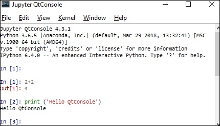
You get a terminal similar to IPython terminal with first In[] prompt. You can now execute any Python expression exactly like we do in IPython terminal or Jupyter notebook
Jupyter QtConsole - Multiline Editing
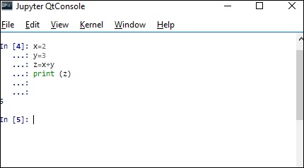
Multiline editing is one of the features which is not available in IPython terminal. In order to enter more than one statements in a single input cell, press ctrl+enter after the first line. Subsequently, just pressing enter will go on adding new line in the same cell. To stop entering new lines and running cell, press enter key one more time at the end. The cell will run and output will be displayed in next out[] cell.
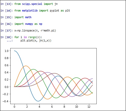
Jupyter QtConsole - Inline Graphics
Another important enhancement offered by QtConsole is the ability to display inline graphics, especially plots. The feature works well with Matplotlib as well as other plotting libraries.
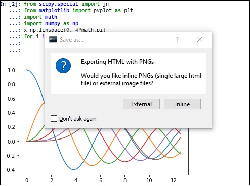
Jupyter QtConsole - Save to HTML
This option to save the QtConsole output as HTML file is available in File menu. You can choose to create file with inline image or the plotted figure as external png file in an adjacent folder (named as qt_files).
Jupyter QtConsole - Multiple Consoles
You can open more than one tabs in Jupyter console application. Three options in File menu are provided for this purpose.
New Tab with New kernel − You can load a new kernel with this file menu.
New Tab with Existing kernel − Using this option, you can choose from additional kernels apart from IPython kernel.
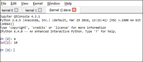
New Tab with Same Kernel − This creates a slave of kernel loaded on a particular tab. As a result, object initialized on master tab will be accessible in slave and vice versa.
Connecting to Jupyter Notebook
There is a %qtconsole magic command available for use with Jupyter notebook. This invokes the QtConsole as a slave terminal to notebook frontend. As a result, data between notebook and Qtconsole terminal can be shared.
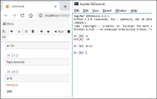
You can see that the variable in notebook is accessible within qtconsole window. Also, a new variable in Qtconsole is used back in notebook.
Observe that the input and output cells are numbered incrementally between the two.
Using github and nbviewer
Sharing Jupyter notebook – Using github and nbviewer
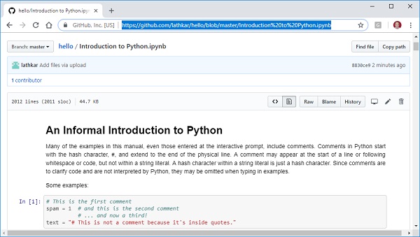
Jupyter Notebook files with .ipynb extension in a GitHub repository will be rendered as static HTML files when they are opened. The interactive features of the notebook, such as custom JavaScript plots, will not work in your repository on GitHub.
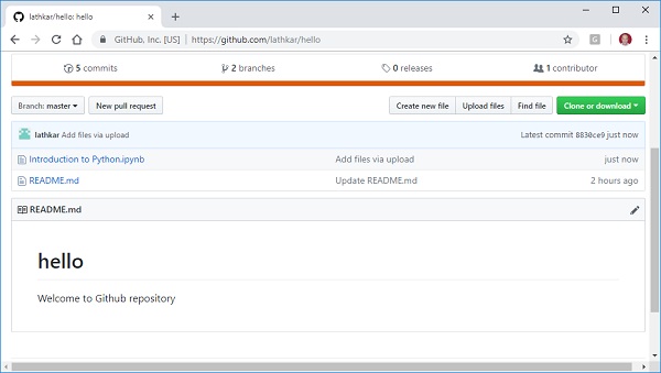
To share notebook file using github, login to https://github.comand create a public repository. Then upload your files using upload file button as shown below −
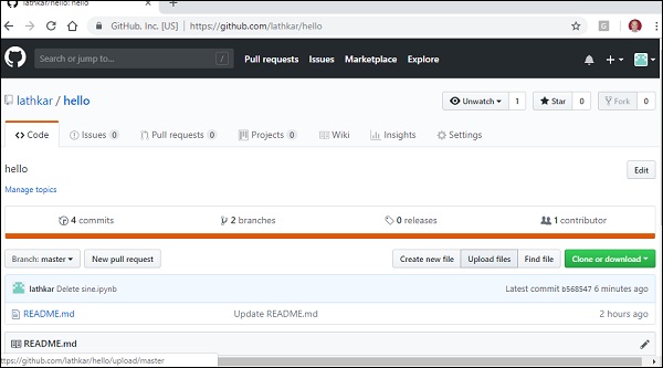
This will give you an option to commit the changes made to the repository. Then, the repository will show uploaded file as below −
Click on the uploaded file to view inside github viewer. You can share the highlighted URL to others.
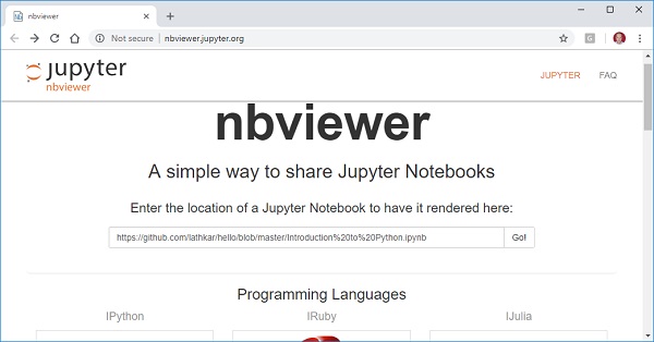
Another way to view the notebook file online is by using nbviewer utility of Project Jupyter. Open https://nbviewer.jupyter.org/ and put URL of file in your repository in the textfield as shown. Press Go button to view the notebook.
Both these methods display notebook file as static html. To be able to execute code in the notebook, open it using Binder application of Jupyter project.
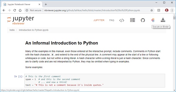
In the nbviewer window you will see ‘Execute on Binder’ button. Click on it and you will see the notebook file opened exactly like you open it from local dashboard of notebook server on your local machine. You can perform all actions like add/edit cells, run the cells etc.
JupyterLab - Overview
Project Jupyter describes JupyterLab as a next generation web based user interfaces for all products under the Jupyter ecosystem. It enables you to work seamlessly with notebook, editors and terminals in an extensible manner.
Some of the important features of JupyterLab are discussed below −
Code Console acts as scratchpad for running code interactively. It has full support for rich output and can be linked to a notebook kernel to log notebook activity.
Any text file (Markdown, Python, R, LaTeX, etc.) can be run interactively in any Jupyter kernel.
Notebook cell output can be shown into its own tab, or along with the notebook, enabling simple dashboards with interactive controls backed by a kernel.
Live editing of document reflects in other viewers such as editors or consoles. It is possible to have live preview of Markdown, Delimiter-separated Values, or Vega/Vega-Lite documents.
JupyterLab can handle many file formats (images, CSV, JSON, Markdown, PDF etc.). It also displays rich output in these formats. JupyterLab provides customizable keyboard shortcuts uses key maps from many well-known text editors.
JupyterLab - Installation and Getting Started
You can try online the features of JupyterLab before installing. Visit https://jupyter.org/try and choose ‘try JupyterLab’ option.
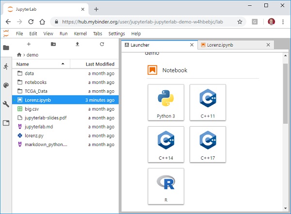
The launcher tab shows currently available kernels and consoles. You can start a new notebook based/terminal based on any of them. The left column is also having tabs for file browser, running kernels and tabs and settings view.
JupyterLab is normally installed automatically with Anaconda distribution. However, it can also be installed separately by using following conda command −
conda install -c conda-forge jupyterlab
You can also use the pip command for this purpose −
pip3 install jupyterlab
To start JupyterLab application, most convenient way is from Anaconda Navigator if it is installed.
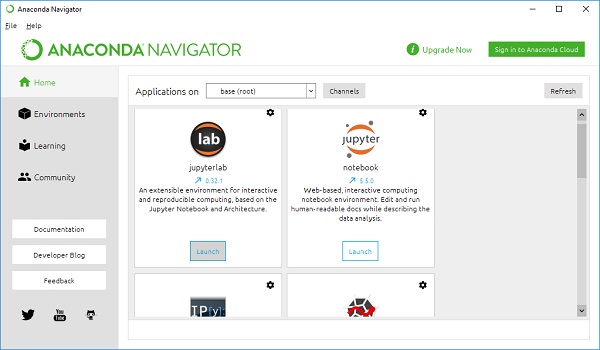
Alternately start it from command line from Windows/Linux command terminal or Anaconda prompt using this command −
jupyter lab
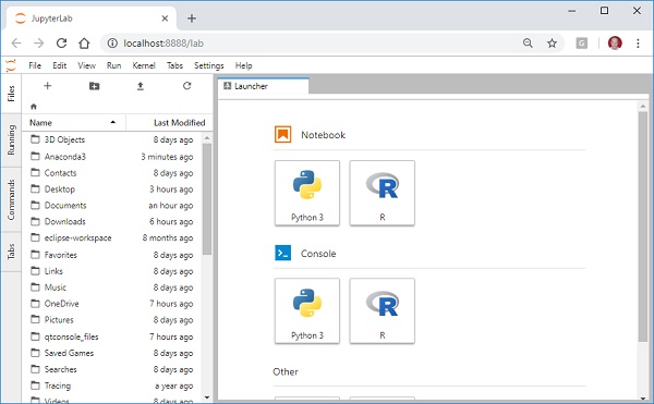
Either way, the JupyterLab application’s launch screen looks like this −
JupyterLab - Interface
To start a new notebook, click the desired kernel. In above screenshot, one kernel is seen that is Python3 kernel. Click it to start a Python notebook. Observe that its functionality is similar to the one we have studied in this tutorial.
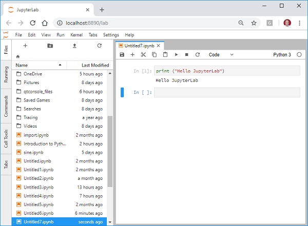
Menu Bar
The menu bar is at the top of window. The default menus you can find in this are −
File − Actions related to files and directories.
Edit − Actions related to editing documents and other activities.
View − Actions that alter the appearance of JupyterLab.
Run − Actions for running code in different activities such as notebooks and code consoles.
Kernel − Actions for managing kernels, which are separate processes for running code.
Tabs − A list of the open documents and activities in the dock panel.
Settings − Common settings and an advanced settings editor.
Help − A list of JupyterLab and kernel help links.
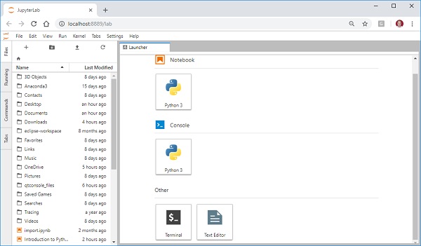
The left sidebar shows buttons for starting a new launcher, adding a folder, uploading file and refresh file list. The right pane is the main working area where notebook, console and terminals are shown in tabbed view.
To start a new console, click + symbol in the left side bar to open a new launcher and then click the console option. The console will open in new tab on the right pane.
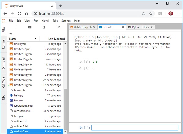
Note that the input cell is at the bottom, but when it is run, the cell and its corresponding output cell appears in upper part of console tab.
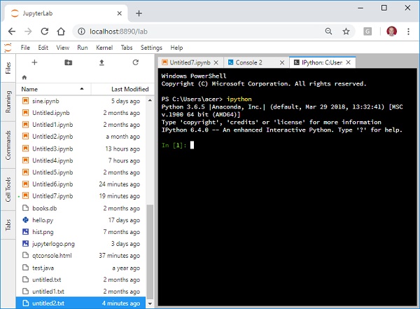
The launcher also allows you open a text editor and a terminal in which IPython shell can be invoked.
JupyterLab - Installing R Kernel
Project Jupyter now supports kernels of programming environments. We shall now see how to install R kernel in anaconda distribution.
In Anaconda prompt window enter following command −
conda install -c r r-essentials
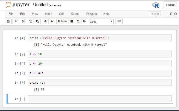
Now, from the launcher tab, choose R kernel to start a new notebook.
The following is a screenshot of Jupyter notebook having R kernel −