- Graph Theory Tutorial
- Graph Theory - Home
- Graph Theory - Introduction
- Graph Theory - Fundamentals
- Graph Theory - Basic Properties
- Graph Theory - Types of Graphs
- Graph Theory - Trees
- Graph Theory - Connectivity
- Graph Theory - Coverings
- Graph Theory - Matchings
- Graph Theory - Independent Sets
- Graph Theory - Coloring
- Graph Theory - Isomorphism
- Graph Theory - Traversability
- Graph Theory - Examples
- Graph Theory Useful Resources
- Graph Theory - Quick Guide
- Graph Theory - Useful Resources
- Graph Theory - Discussion
Graph Theory - Quick Guide
Graph Theory - Introduction
In the domain of mathematics and computer science, graph theory is the study of graphs that concerns with the relationship among edges and vertices. It is a popular subject having its applications in computer science, information technology, biosciences, mathematics, and linguistics to name a few. Without further ado, let us start with defining a graph.
What is a Graph?
A graph is a pictorial representation of a set of objects where some pairs of objects are connected by links. The interconnected objects are represented by points termed as vertices, and the links that connect the vertices are called edges.
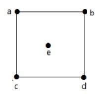
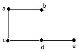
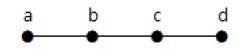
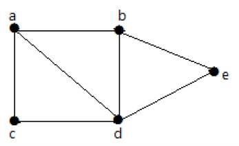
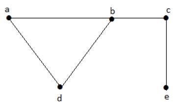
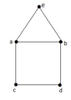
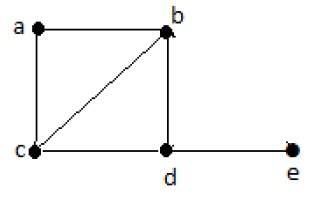
Formally, a graph is a pair of sets (V, E), where V is the set of vertices and E is the set of edges, connecting the pairs of vertices. Take a look at the following graph −
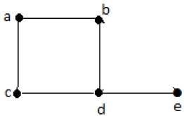
In the above graph,
V = {a, b, c, d, e}
E = {ab, ac, bd, cd, de}
Applications of Graph Theory
Graph theory has its applications in diverse fields of engineering −
Electrical Engineering − The concepts of graph theory is used extensively in designing circuit connections. The types or organization of connections are named as topologies. Some examples for topologies are star, bridge, series, and parallel topologies.
Computer Science − Graph theory is used for the study of algorithms. For example,
- Kruskal's Algorithm
- Prim's Algorithm
- Dijkstra's Algorithm
Computer Network − The relationships among interconnected computers in the network follows the principles of graph theory.
Science − The molecular structure and chemical structure of a substance, the DNA structure of an organism, etc., are represented by graphs.
Linguistics − The parsing tree of a language and grammar of a language uses graphs.
General − Routes between the cities can be represented using graphs. Depicting hierarchical ordered information such as family tree can be used as a special type of graph called tree.
Graph Theory - Fundamentals
A graph is a diagram of points and lines connected to the points. It has at least one line joining a set of two vertices with no vertex connecting itself. The concept of graphs in graph theory stands up on some basic terms such as point, line, vertex, edge, degree of vertices, properties of graphs, etc. Here, in this chapter, we will cover these fundamentals of graph theory.
Point
A point is a particular position in a one-dimensional, two-dimensional, or three-dimensional space. For better understanding, a point can be denoted by an alphabet. It can be represented with a dot.
Example

Here, the dot is a point named ‘a’.
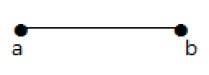
Line
A Line is a connection between two points. It can be represented with a solid line.
Example
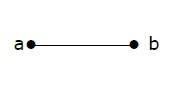
Here, ‘a’ and ‘b’ are the points. The link between these two points is called a line.
Vertex
A vertex is a point where multiple lines meet. It is also called a node. Similar to points, a vertex is also denoted by an alphabet.
Example

Here, the vertex is named with an alphabet ‘a’.
Edge
An edge is the mathematical term for a line that connects two vertices. Many edges can be formed from a single vertex. Without a vertex, an edge cannot be formed. There must be a starting vertex and an ending vertex for an edge.
Example
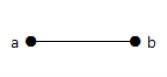
Here, ‘a’ and ‘b’ are the two vertices and the link between them is called an edge.
Graph
A graph ‘G’ is defined as G = (V, E) Where V is a set of all vertices and E is a set of all edges in the graph.
Example 1
In the above example, ab, ac, cd, and bd are the edges of the graph. Similarly, a, b, c, and d are the vertices of the graph.
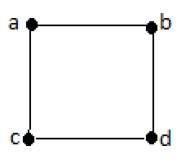
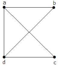
Example 2
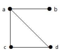
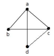
In this graph, there are four vertices a, b, c, and d, and four edges ab, ac, ad, and cd.
Loop
In a graph, if an edge is drawn from vertex to itself, it is called a loop.
Example 1
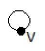
In the above graph, V is a vertex for which it has an edge (V, V) forming a loop.
Example 2
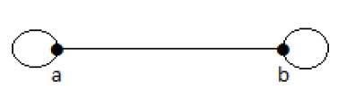
In this graph, there are two loops which are formed at vertex a, and vertex b.
Degree of Vertex
It is the number of vertices adjacent to a vertex V.
Notation − deg(V).
In a simple graph with n number of vertices, the degree of any vertices is −
deg(v) ≤ n – 1 ∀ v ∈ G
A vertex can form an edge with all other vertices except by itself. So the degree of a vertex will be up to the number of vertices in the graph minus 1. This 1 is for the self-vertex as it cannot form a loop by itself. If there is a loop at any of the vertices, then it is not a Simple Graph.
Degree of vertex can be considered under two cases of graphs −
Undirected Graph
Directed Graph
Degree of Vertex in an Undirected Graph
An undirected graph has no directed edges. Consider the following examples.
Example 1
Take a look at the following graph −
In the above Undirected Graph,
deg(a) = 2, as there are 2 edges meeting at vertex ‘a’.
deg(b) = 3, as there are 3 edges meeting at vertex ‘b’.
deg(c) = 1, as there is 1 edge formed at vertex ‘c’
So ‘c’ is a pendent vertex.
deg(d) = 2, as there are 2 edges meeting at vertex ‘d’.
deg(e) = 0, as there are 0 edges formed at vertex ‘e’.
So ‘e’ is an isolated vertex.
Example 2
Take a look at the following graph −
In the above graph,
deg(a) = 2, deg(b) = 2, deg(c) = 2, deg(d) = 2, and deg(e) = 0.
The vertex ‘e’ is an isolated vertex. The graph does not have any pendent vertex.
Degree of Vertex in a Directed Graph
In a directed graph, each vertex has an indegree and an outdegree.
Indegree of a Graph
Indegree of vertex V is the number of edges which are coming into the vertex V.
Notation − deg−(V).
Outdegree of a Graph
Outdegree of vertex V is the number of edges which are going out from the vertex V.
Notation − deg+(V).
Consider the following examples.
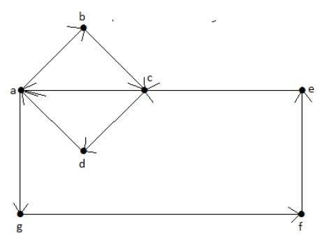
Example 1
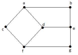
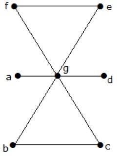
Take a look at the following directed graph. Vertex ‘a’ has two edges, ‘ad’ and ‘ab’, which are going outwards. Hence its outdegree is 2. Similarly, there is an edge ‘ga’, coming towards vertex ‘a’. Hence the indegree of ‘a’ is 1.
The indegree and outdegree of other vertices are shown in the following table −
| Vertex | Indegree | Outdegree |
|---|---|---|
| a | 1 | 2 |
| b | 2 | 0 |
| c | 2 | 1 |
| d | 1 | 1 |
| e | 1 | 1 |
| f | 1 | 1 |
| g | 0 | 2 |
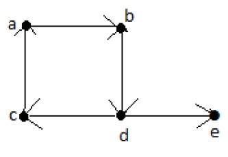
Example 2
Take a look at the following directed graph. Vertex ‘a’ has an edge ‘ae’ going outwards from vertex ‘a’. Hence its outdegree is 1. Similarly, the graph has an edge ‘ba’ coming towards vertex ‘a’. Hence the indegree of ‘a’ is 1.
The indegree and outdegree of other vertices are shown in the following table −
| Vertex | Indegree | Outdegree |
|---|---|---|
| a | 1 | 1 |
| b | 0 | 2 |
| c | 2 | 0 |
| d | 1 | 1 |
| e | 1 | 1 |
Pendent Vertex
By using degree of a vertex, we have a two special types of vertices. A vertex with degree one is called a pendent vertex.
Example
Here, in this example, vertex ‘a’ and vertex ‘b’ have a connected edge ‘ab’. So with respect to the vertex ‘a’, there is only one edge towards vertex ‘b’ and similarly with respect to the vertex ‘b’, there is only one edge towards vertex ‘a’. Finally, vertex ‘a’ and vertex ‘b’ has degree as one which are also called as the pendent vertex.
Isolated Vertex
A vertex with degree zero is called an isolated vertex.
Example
Here, the vertex ‘a’ and vertex ‘b’ has a no connectivity between each other and also to any other vertices. So the degree of both the vertices ‘a’ and ‘b’ are zero. These are also called as isolated vertices.
Adjacency
Here are the norms of adjacency −
In a graph, two vertices are said to be adjacent, if there is an edge between the two vertices. Here, the adjacency of vertices is maintained by the single edge that is connecting those two vertices.
In a graph, two edges are said to be adjacent, if there is a common vertex between the two edges. Here, the adjacency of edges is maintained by the single vertex that is connecting two edges.
Example 1
In the above graph −
‘a’ and ‘b’ are the adjacent vertices, as there is a common edge ‘ab’ between them.
‘a’ and ‘d’ are the adjacent vertices, as there is a common edge ‘ad’ between them.
ab’ and ‘be’ are the adjacent edges, as there is a common vertex ‘b’ between them.
be’ and ‘de’ are the adjacent edges, as there is a common vertex ‘e’ between them.
Example 2
In the above graph −
‘a’ and ‘d’ are the adjacent vertices, as there is a common edge ‘ad’ between them.
‘c’ and ‘b’ are the adjacent vertices, as there is a common edge ‘cb’ between them.
‘ad’ and ‘cd’ are the adjacent edges, as there is a common vertex ‘d’ between them.
‘ac’ and ‘cd’ are the adjacent edges, as there is a common vertex ‘c’ between them.
Parallel Edges
In a graph, if a pair of vertices is connected by more than one edge, then those edges are called parallel edges.
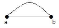
In the above graph, ‘a’ and ‘b’ are the two vertices which are connected by two edges ‘ab’ and ‘ab’ between them. So it is called as a parallel edge.
Multi Graph
A graph having parallel edges is known as a Multigraph.
Example 1
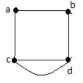
In the above graph, there are five edges ‘ab’, ‘ac’, ‘cd’, ‘cd’, and ‘bd’. Since ‘c’ and ‘d’ have two parallel edges between them, it a Multigraph.
Example 2
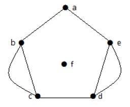
In the above graph, the vertices ‘b’ and ‘c’ have two edges. The vertices ‘e’ and ‘d’ also have two edges between them. Hence it is a Multigraph.
Degree Sequence of a Graph
If the degrees of all vertices in a graph are arranged in descending or ascending order, then the sequence obtained is known as the degree sequence of the graph.
Example 1
| Vertex | A | b | c | d | e |
|---|---|---|---|---|---|
| Connecting to | b,c | a,d | a,d | c,b,e | d |
| Degree | 2 | 2 | 2 | 3 | 1 |
In the above graph, for the vertices {d, a, b, c, e}, the degree sequence is {3, 2, 2, 2, 1}.
Example 2
| Vertex | A | b | c | d | e | f |
|---|---|---|---|---|---|---|
| Connecting to | b,e | a,c | b,d | c,e | a,d | - |
| Degree | 2 | 2 | 2 | 2 | 2 | 0 |
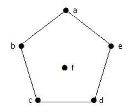
In the above graph, for the vertices {a, b, c, d, e, f}, the degree sequence is {2, 2, 2, 2, 2, 0}.
Graph Theory - Basic Properties
Graphs come with various properties which are used for characterization of graphs depending on their structures. These properties are defined in specific terms pertaining to the domain of graph theory. In this chapter, we will discuss a few basic properties that are common in all graphs.
Distance between Two Vertices
It is number of edges in a shortest path between Vertex U and Vertex V. If there are multiple paths connecting two vertices, then the shortest path is considered as the distance between the two vertices.
Notation − d(U,V)
There can be any number of paths present from one vertex to other. Among those, you need to choose only the shortest one.
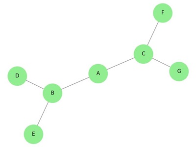
Example
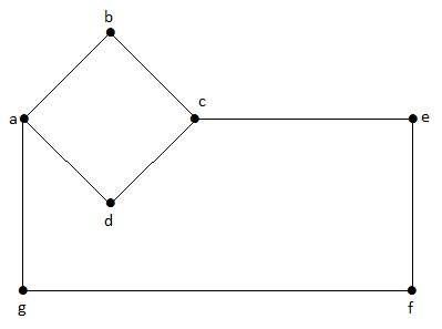
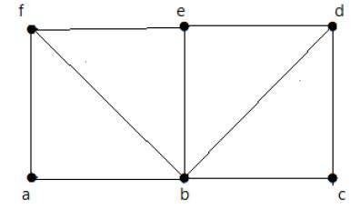
Take a look at the following graph −
Here, the distance from vertex ‘d’ to vertex ‘e’ or simply ‘de’ is 1 as there is one edge between them. There are many paths from vertex ‘d’ to vertex ‘e’ −
- da, ab, be
- df, fg, ge
- de (It is considered for distance between the vertices)
- df, fc, ca, ab, be
- da, ac, cf, fg, ge
Eccentricity of a Vertex
The maximum distance between a vertex to all other vertices is considered as the eccentricity of vertex.
Notation − e(V)
The distance from a particular vertex to all other vertices in the graph is taken and among those distances, the eccentricity is the highest of distances.
Example
In the above graph, the eccentricity of ‘a’ is 3.
The distance from ‘a’ to ‘b’ is 1 (‘ab’),
from ‘a’ to ‘c’ is 1 (‘ac’),
from ‘a’ to ‘d’ is 1 (‘ad’),
from ‘a’ to ‘e’ is 2 (‘ab’-‘be’) or (‘ad’-‘de’),
from ‘a’ to ‘f’ is 2 (‘ac’-‘cf’) or (‘ad’-‘df’),
from ‘a’ to ‘g’ is 3 (‘ac’-‘cf’-‘fg’) or (‘ad’-‘df’-‘fg’).
So the eccentricity is 3, which is a maximum from vertex ‘a’ from the distance between ‘ag’ which is maximum.
In other words,
e(b) = 3
e(c) = 3
e(d) = 2
e(e) = 3
e(f) = 3
e(g) = 3
Radius of a Connected Graph
The minimum eccentricity from all the vertices is considered as the radius of the Graph G. The minimum among all the maximum distances between a vertex to all other vertices is considered as the radius of the Graph G.
Notation − r(G)
From all the eccentricities of the vertices in a graph, the radius of the connected graph is the minimum of all those eccentricities.
Example
In the above graph r(G) = 2, which is the minimum eccentricity for ‘d’.
Diameter of a Graph
The maximum eccentricity from all the vertices is considered as the diameter of the Graph G. The maximum among all the distances between a vertex to all other vertices is considered as the diameter of the Graph G.
Notation − d(G) − From all the eccentricities of the vertices in a graph, the diameter of the connected graph is the maximum of all those eccentricities.
Example
In the above graph, d(G) = 3; which is the maximum eccentricity.
Central Point
If the eccentricity of a graph is equal to its radius, then it is known as the central point of the graph. If
e(V) = r(V),
then ‘V’ is the central point of the Graph ’G’.
Example
In the example graph, ‘d’ is the central point of the graph.
e(d) = r(d) = 2
Centre
The set of all central points of ‘G’ is called the centre of the Graph.
Example
In the example graph, {‘d’} is the centre of the Graph.
Circumference
The number of edges in the longest cycle of ‘G’ is called as the circumference of ‘G’.
Example
In the example graph, the circumference is 6, which we derived from the longest cycle a-c-f-g-e-b-a or a-c-f-d-e-b-a.
Girth
The number of edges in the shortest cycle of ‘G’ is called its Girth.
Notation: g(G).
Example − In the example graph, the Girth of the graph is 4, which we derived from the shortest cycle a-c-f-d-a or d-f-g-e-d or a-b-e-d-a.
Sum of Degrees of Vertices Theorem
If G = (V, E) be a non-directed graph with vertices V = {V1, V2,…Vn} then
Corollary 1
If G = (V, E) be a directed graph with vertices V = {V1, V2,…Vn}, then
Corollary 2
In any non-directed graph, the number of vertices with Odd degree is Even.
Corollary 3
In a non-directed graph, if the degree of each vertex is k, then
Corollary 4
In a non-directed graph, if the degree of each vertex is at least k, then
| Corollary 5
In a non-directed graph, if the degree of each vertex is at most k, then
Graph Theory - Types of Graphs
There are various types of graphs depending upon the number of vertices, number of edges, interconnectivity, and their overall structure. We will discuss only a certain few important types of graphs in this chapter.
Null Graph
A graph having no edges is called a Null Graph.
Example
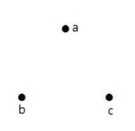
In the above graph, there are three vertices named ‘a’, ‘b’, and ‘c’, but there are no edges among them. Hence it is a Null Graph.
Trivial Graph
A graph with only one vertex is called a Trivial Graph.
Example
In the above shown graph, there is only one vertex ‘a’ with no other edges. Hence it is a Trivial graph.
Non-Directed Graph
A non-directed graph contains edges but the edges are not directed ones.
Example
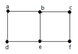
In this graph, ‘a’, ‘b’, ‘c’, ‘d’, ‘e’, ‘f’, ‘g’ are the vertices, and ‘ab’, ‘bc’, ‘cd’, ‘da’, ‘ag’, ‘gf’, ‘ef’ are the edges of the graph. Since it is a non-directed graph, the edges ‘ab’ and ‘ba’ are same. Similarly other edges also considered in the same way.
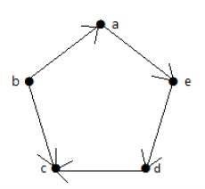
Directed Graph
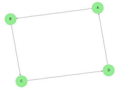
In a directed graph, each edge has a direction.
Example
In the above graph, we have seven vertices ‘a’, ‘b’, ‘c’, ‘d’, ‘e’, ‘f’, and ‘g’, and eight edges ‘ab’, ‘cb’, ‘dc’, ‘ad’, ‘ec’, ‘fe’, ‘gf’, and ‘ga’. As it is a directed graph, each edge bears an arrow mark that shows its direction. Note that in a directed graph, ‘ab’ is different from ‘ba’.
Simple Graph
A graph with no loops and no parallel edges is called a simple graph.
The maximum number of edges possible in a single graph with ‘n’ vertices is nC2 where nC2 = n(n – 1)/2.
The number of simple graphs possible with ‘n’ vertices = 2nc2 = 2n(n-1)/2.
Example
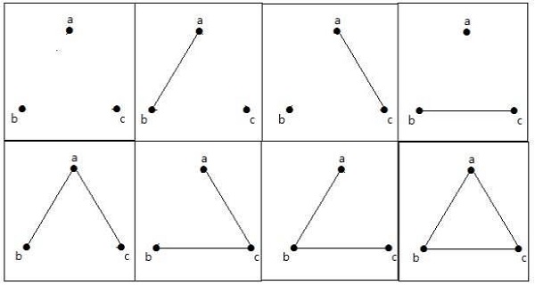
In the following graph, there are 3 vertices with 3 edges which is maximum excluding the parallel edges and loops. This can be proved by using the above formulae.
The maximum number of edges with n=3 vertices −
The maximum number of simple graphs with n=3 vertices −
These 8 graphs are as shown below −
Connected Graph
A graph G is said to be connected if there exists a path between every pair of vertices. There should be at least one edge for every vertex in the graph. So that we can say that it is connected to some other vertex at the other side of the edge.
Example
In the following graph, each vertex has its own edge connected to other edge. Hence it is a connected graph.
Disconnected Graph
A graph G is disconnected, if it does not contain at least two connected vertices.
Example 1
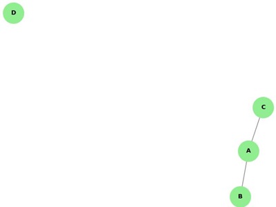
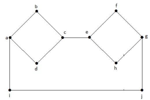
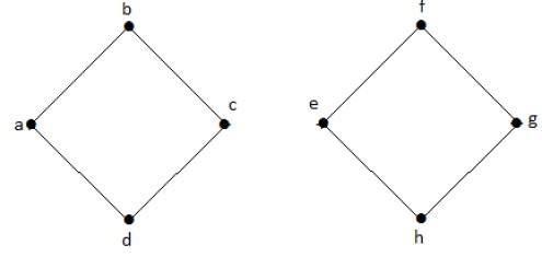
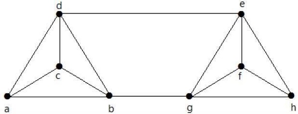
The following graph is an example of a Disconnected Graph, where there are two components, one with ‘a’, ‘b’, ‘c’, ‘d’ vertices and another with ‘e’, ’f’, ‘g’, ‘h’ vertices.
The two components are independent and not connected to each other. Hence it is called disconnected graph.
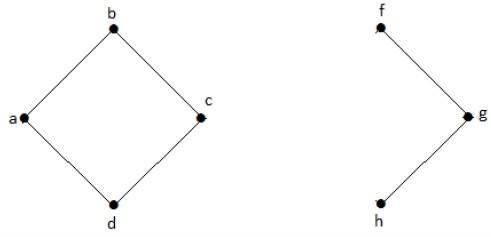
Example 2
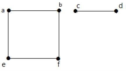
In this example, there are two independent components, a-b-f-e and c-d, which are not connected to each other. Hence this is a disconnected graph.
Regular Graph
A graph G is said to be regular, if all its vertices have the same degree. In a graph, if the degree of each vertex is ‘k’, then the graph is called a ‘k-regular graph’.
Example
In the following graphs, all the vertices have the same degree. So these graphs are called regular graphs.
In both the graphs, all the vertices have degree 2. They are called 2-Regular Graphs.
Complete Graph
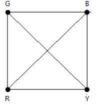
A simple graph with ‘n’ mutual vertices is called a complete graph and it is denoted by ‘Kn’. In the graph, a vertex should have edges with all other vertices, then it called a complete graph.
In other words, if a vertex is connected to all other vertices in a graph, then it is called a complete graph.
Example
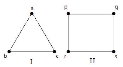
In the following graphs, each vertex in the graph is connected with all the remaining vertices in the graph except by itself.
In graph I,
| a | b | c | |
|---|---|---|---|
| a | Not Connected | Connected | Connected |
| b | Connected | Not Connected | Connected |
| c | Connected | Connected | Not Connected |
In graph II,
| p | q | r | s | |
|---|---|---|---|---|
| p | Not Connected | Connected | Connected | Connected |
| q | Connected | Not Connected | Connected | Connected |
| r | Connected | Connected | Not Connected | Connected |
| s | Connected | Connected | Connected | Not Connected |
Cycle Graph
A simple graph with ‘n’ vertices (n >= 3) and ‘n’ edges is called a cycle graph if all its edges form a cycle of length ‘n’.
If the degree of each vertex in the graph is two, then it is called a Cycle Graph.
Notation − Cn
Example
Take a look at the following graphs −
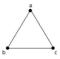
Graph I has 3 vertices with 3 edges which is forming a cycle ‘ab-bc-ca’.
Graph II has 4 vertices with 4 edges which is forming a cycle ‘pq-qs-sr-rp’.
Graph III has 5 vertices with 5 edges which is forming a cycle ‘ik-km-ml-lj-ji’.
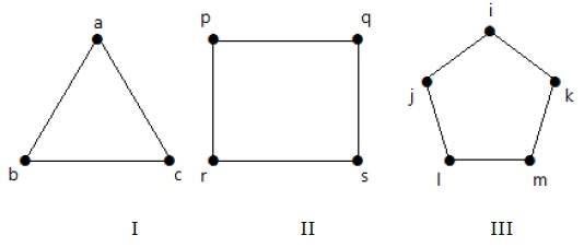
Hence all the given graphs are cycle graphs.
Wheel Graph
A wheel graph is obtained from a cycle graph Cn-1 by adding a new vertex. That new vertex is called a Hub which is connected to all the vertices of Cn.
Notation − Wn
No. of edges in Wn = No. of edges from hub to all other vertices +
No. of edges from all other nodes in cycle graph without a hub.
= (n–1) + (n–1)
= 2(n–1)
Example
Take a look at the following graphs. They are all wheel graphs.
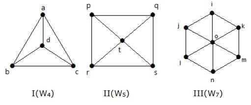
In graph I, it is obtained from C3 by adding an vertex at the middle named as ‘d’. It is denoted as W4.
Number of edges in W4 = 2(n-1) = 2(3) = 6
In graph II, it is obtained from C4 by adding a vertex at the middle named as ‘t’. It is denoted as W5.
Number of edges in W5 = 2(n-1) = 2(4) = 8
In graph III, it is obtained from C6 by adding a vertex at the middle named as ‘o’. It is denoted as W7.
Number of edges in W4 = 2(n-1) = 2(6) = 12
Cyclic Graph
A graph with at least one cycle is called a cyclic graph.
Example
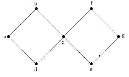
In the above example graph, we have two cycles a-b-c-d-a and c-f-g-e-c. Hence it is called a cyclic graph.
Acyclic Graph
A graph with no cycles is called an acyclic graph.
Example
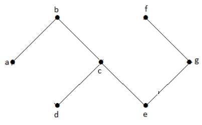
In the above example graph, we do not have any cycles. Hence it is a non-cyclic graph.
Bipartite Graph
A simple graph G = (V, E) with vertex partition V = {V1, V2} is called a bipartite graph if every edge of E joins a vertex in V1 to a vertex in V2.
In general, a Bipertite graph has two sets of vertices, let us say, V1 and V2, and if an edge is drawn, it should connect any vertex in set V1 to any vertex in set V2.
Example
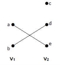
In this graph, you can observe two sets of vertices − V1 and V2. Here, two edges named ‘ae’ and ‘bd’ are connecting the vertices of two sets V1 and V2.
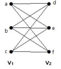
Complete Bipartite Graph
A bipartite graph ‘G’, G = (V, E) with partition V = {V1, V2} is said to be a complete bipartite graph if every vertex in V1 is connected to every vertex of V2.
In general, a complete bipartite graph connects each vertex from set V1 to each vertex from set V2.
Example
The following graph is a complete bipartite graph because it has edges connecting each vertex from set V1 to each vertex from set V2.
If |V1| = m and |V2| = n, then the complete bipartite graph is denoted by Km, n.
- Km,n has (m+n) vertices and (mn) edges.
- Km,n is a regular graph if m=n.
In general, a complete bipartite graph is not a complete graph.
Km,n is a complete graph if m=n=1.
The maximum number of edges in a bipartite graph with n vertices is −
[n2/4]
If n=10, k5, 5= [n2/4] = [102/4] = 25.
Similarly, K6, 4=24
K7, 3=21
K8, 2=16
K9, 1=9
If n=9, k5, 4 = [n2/4] = [92/4] = 20
Similarly, K6, 3=18
K7, 2=14
K8, 1=8
‘G’ is a bipartite graph if ‘G’ has no cycles of odd length. A special case of bipartite graph is a star graph.
Star Graph
A complete bipartite graph of the form K1, n-1 is a star graph with n-vertices. A star graph is a complete bipartite graph if a single vertex belongs to one set and all the remaining vertices belong to the other set.
Example
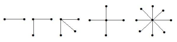
In the above graphs, out of ‘n’ vertices, all the ‘n–1’ vertices are connected to a single vertex. Hence it is in the form of K1, n-1 which are star graphs.
Complement of a Graph
Let 'G−' be a simple graph with some vertices as that of ‘G’ and an edge {U, V} is present in 'G−', if the edge is not present in G. It means, two vertices are adjacent in 'G−' if the two vertices are not adjacent in G.
If the edges that exist in graph I are absent in another graph II, and if both graph I and graph II are combined together to form a complete graph, then graph I and graph II are called complements of each other.
Example
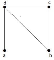
In the following example, graph-I has two edges ‘cd’ and ‘bd’. Its complement graph-II has four edges.
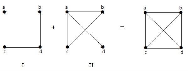
Note that the edges in graph-I are not present in graph-II and vice versa. Hence, the combination of both the graphs gives a complete graph of ‘n’ vertices.
Note − A combination of two complementary graphs gives a complete graph.
If ‘G’ is any simple graph, then
|E(G)| + |E('G-')| = |E(Kn)|, where n = number of vertices in the graph.
Example
Let ‘G’ be a simple graph with nine vertices and twelve edges, find the number of edges in 'G-'.
You have, |E(G)| + |E('G-')| = |E(Kn)|
12 + |E('G-')| =
9(9-1) / 2 = 9C2
12 + |E('G-')| = 36
|E('G-')| = 24
‘G’ is a simple graph with 40 edges and its complement 'G−' has 38 edges. Find the number of vertices in the graph G or 'G−'.
Let the number of vertices in the graph be ‘n’.
We have, |E(G)| + |E('G-')| = |E(Kn)|
40 + 38 = n(n-1)/2
156 = n(n-1)
13(12) = n(n-1)
n = 13
Graph Theory - Trees
Trees are graphs that do not contain even a single cycle. They represent hierarchical structure in a graphical form. Trees belong to the simplest class of graphs. Despite their simplicity, they have a rich structure.
Trees provide a range of useful applications as simple as a family tree to as complex as trees in data structures of computer science.
Tree
A connected acyclic graph is called a tree. In other words, a connected graph with no cycles is called a tree.
The edges of a tree are known as branches. Elements of trees are called their nodes. The nodes without child nodes are called leaf nodes.
A tree with ‘n’ vertices has ‘n-1’ edges. If it has one more edge extra than ‘n-1’, then the extra edge should obviously has to pair up with two vertices which leads to form a cycle. Then, it becomes a cyclic graph which is a violation for the tree graph.
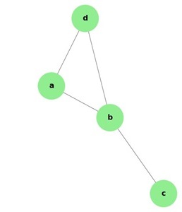
Example 1
The graph shown here is a tree because it has no cycles and it is connected. It has four vertices and three edges, i.e., for ‘n’ vertices ‘n-1’ edges as mentioned in the definition.
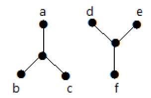
Note − Every tree has at least two vertices of degree one.
Example 2
In the above example, the vertices ‘a’ and ‘d’ has degree one. And the other two vertices ‘b’ and ‘c’ has degree two. This is possible because for not forming a cycle, there should be at least two single edges anywhere in the graph. It is nothing but two edges with a degree of one.
Forest
A disconnected acyclic graph is called a forest. In other words, a disjoint collection of trees is called a forest.
Example
The following graph looks like two sub-graphs; but it is a single disconnected graph. There are no cycles in this graph. Hence, clearly it is a forest.
Spanning Trees
Let G be a connected graph, then the sub-graph H of G is called a spanning tree of G if −
- H is a tree
- H contains all vertices of G.
A spanning tree T of an undirected graph G is a subgraph that includes all of the vertices of G.
Example
In the above example, G is a connected graph and H is a sub-graph of G.
Clearly, the graph H has no cycles, it is a tree with six edges which is one less than the total number of vertices. Hence H is the Spanning tree of G.
Circuit Rank
Let ‘G’ be a connected graph with ‘n’ vertices and ‘m’ edges. A spanning tree ‘T’ of G contains (n-1) edges.
Therefore, the number of edges you need to delete from ‘G’ in order to get a spanning tree = m-(n-1), which is called the circuit rank of G.
This formula is true, because in a spanning tree you need to have ‘n-1’ edges. Out of ‘m’ edges, you need to keep ‘n–1’ edges in the graph.
Hence, deleting ‘n–1’ edges from ‘m’ gives the edges to be removed from the graph in order to get a spanning tree, which should not form a cycle.
Example
Take a look at the following graph −
For the graph given in the above example, you have m=7 edges and n=5 vertices.
Then the circuit rank is −
Example
Let ‘G’ be a connected graph with six vertices and the degree of each vertex is three. Find the circuit rank of ‘G’.
By the sum of degree of vertices theorem,
Kirchoff’s Theorem
Kirchoff’s theorem is useful in finding the number of spanning trees that can be formed from a connected graph.
Example
The matrix ‘A’ be filled as, if there is an edge between two vertices, then it should be given as ‘1’, else ‘0’.
$$A=\begin{vmatrix}0 & a & b & c & d\\a & 0 & 1 & 1 & 1 \\b & 1 & 0 & 0 & 1\\c & 1 & 0 & 0 & 1\\d & 1 & 1 & 1 & 0 \end{vmatrix} = \begin{vmatrix} 0 & 1 & 1 & 1\\1 & 0 & 0 & 1\\1 & 0 & 0 & 1\\1 & 1 & 1 & 0\end{vmatrix}$$By using kirchoff's theorem, it should be changed as replacing the principle diagonal values with the degree of vertices and all other elements with -1.A
$$=\begin{vmatrix} 3 & -1 & -1 & -1\\-1 & 2 & 0 & -1\\-1 & 0 & 2 & -1\\-1 & -1 & -1 & 3 \end{vmatrix}=M$$ $$M=\begin{vmatrix}3 & -1 & -1 & -1\\-1 & 2 & 0 & -1\\-1 & 0 & 2 & -1\\-1 & -1 & -1 & 3 \end{vmatrix} =8$$ $$Co\:\:factor\:\:of\:\:m1\:\:= \begin{vmatrix} 2 & 0 & -1\\0 & 2 & -1\\-1 & -1 & 3\end{vmatrix}$$Thus, the number of spanning trees = 8.
Graph Theory - Connectivity
Whether it is possible to traverse a graph from one vertex to another is determined by how a graph is connected. Connectivity is a basic concept in Graph Theory. Connectivity defines whether a graph is connected or disconnected. It has subtopics based on edge and vertex, known as edge connectivity and vertex connectivity. Let us discuss them in detail.
Connectivity
A graph is said to be connected if there is a path between every pair of vertex. From every vertex to any other vertex, there should be some path to traverse. That is called the connectivity of a graph. A graph with multiple disconnected vertices and edges is said to be disconnected.
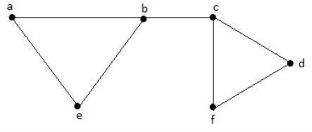
Example 1
In the following graph, it is possible to travel from one vertex to any other vertex. For example, one can traverse from vertex ‘a’ to vertex ‘e’ using the path ‘a-b-e’.
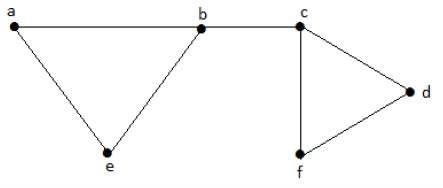
Example 2
In the following example, traversing from vertex ‘a’ to vertex ‘f’ is not possible because there is no path between them directly or indirectly. Hence it is a disconnected graph.
Cut Vertex
Let ‘G’ be a connected graph. A vertex V ∈ G is called a cut vertex of ‘G’, if ‘G-V’ (Delete ‘V’ from ‘G’) results in a disconnected graph. Removing a cut vertex from a graph breaks it in to two or more graphs.
Note − Removing a cut vertex may render a graph disconnected.
A connected graph ‘G’ may have at most (n–2) cut vertices.
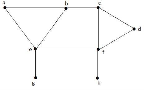
Example
In the following graph, vertices ‘e’ and ‘c’ are the cut vertices.
By removing ‘e’ or ‘c’, the graph will become a disconnected graph.
Without ‘g’, there is no path between vertex ‘c’ and vertex ‘h’ and many other. Hence it is a disconnected graph with cut vertex as ‘e’. Similarly, ‘c’ is also a cut vertex for the above graph.
Cut Edge (Bridge)
Let ‘G’ be a connected graph. An edge ‘e’ ∈ G is called a cut edge if ‘G-e’ results in a disconnected graph.
If removing an edge in a graph results in to two or more graphs, then that edge is called a Cut Edge.
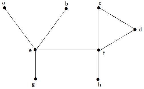
Example
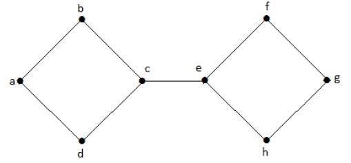
In the following graph, the cut edge is [(c, e)].
By removing the edge (c, e) from the graph, it becomes a disconnected graph.
In the above graph, removing the edge (c, e) breaks the graph into two which is nothing but a disconnected graph. Hence, the edge (c, e) is a cut edge of the graph.
Note − Let ‘G’ be a connected graph with ‘n’ vertices, then
a cut edge e ∈ G if and only if the edge ‘e’ is not a part of any cycle in G.
the maximum number of cut edges possible is ‘n-1’.
whenever cut edges exist, cut vertices also exist because at least one vertex of a cut edge is a cut vertex.
if a cut vertex exists, then a cut edge may or may not exist.
Cut Set of a Graph
Let ‘G’= (V, E) be a connected graph. A subset E’ of E is called a cut set of G if deletion of all the edges of E’ from G makes G disconnect.
If deleting a certain number of edges from a graph makes it disconnected, then those deleted edges are called the cut set of the graph.
Example
Take a look at the following graph. Its cut set is E1 = {e1, e3, e5, e8}.
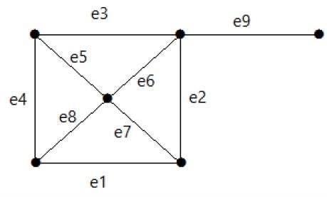
After removing the cut set E1 from the graph, it would appear as follows −
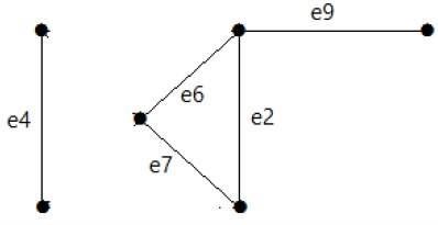
Similarly, there are other cut sets that can disconnect the graph −
E3 = {e9} – Smallest cut set of the graph.
E4 = {e3, e4, e5}
Edge Connectivity
Let ‘G’ be a connected graph. The minimum number of edges whose removal makes ‘G’ disconnected is called edge connectivity of G.
Notation − λ(G)
In other words, the number of edges in a smallest cut set of G is called the edge connectivity of G.
If ‘G’ has a cut edge, then λ(G) is 1. (edge connectivity of G.)
Example
Take a look at the following graph. By removing two minimum edges, the connected graph becomes disconnected. Hence, its edge connectivity (λ(G)) is 2.
Here are the four ways to disconnect the graph by removing two edges −
Vertex Connectivity
Let ‘G’ be a connected graph. The minimum number of vertices whose removal makes ‘G’ either disconnected or reduces ‘G’ in to a trivial graph is called its vertex connectivity.
Notation − K(G)
Example
In the above graph, removing the vertices ‘e’ and ‘i’ makes the graph disconnected.
If G has a cut vertex, then K(G) = 1.
Notation − For any connected graph G,
K(G) ≤ λ(G) ≤ δ(G)
Vertex connectivity (K(G)), edge connectivity (λ(G)), minimum number of degrees of G(δ(G)).
Example
Calculate λ(G) and K(G) for the following graph −
Solution
From the graph,
δ(G) = 3
K(G) ≤ λ(G) ≤ δ(G) = 3 (1)
K(G) ≥ 2 (2)
Deleting the edges {d, e} and {b, h}, we can disconnect G.
Therefore,
λ(G) = 2
2 ≤ λ(G) ≤ δ(G) = 2 (3)
From (2) and (3), vertex connectivity K(G) = 2
Graph Theory - Coverings
A covering graph is a subgraph which contains either all the vertices or all the edges corresponding to some other graph. A subgraph which contains all the vertices is called a line/edge covering. A subgraph which contains all the edges is called a vertex covering.
Line Covering
Let G = (V, E) be a graph. A subset C(E) is called a line covering of G if every vertex of G is incident with at least one edge in C, i.e.,
deg(V) ≥ 1 ∀ V ∈ G
because each vertex is connected with another vertex by an edge. Hence it has a minimum degree of 1.
Example
Take a look at the following graph −
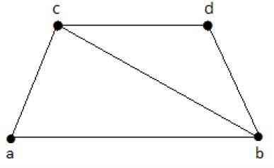
Its subgraphs having line covering are as follows −
C1 = {{a, b}, {c, d}}
C2 = {{a, d}, {b, c}}
C3 = {{a, b}, {b, c}, {b, d}}
C4 = {{a, b}, {b, c}, {c, d}}
Line covering of ‘G’ does not exist if and only if ‘G’ has an isolated vertex. Line covering of a graph with ‘n’ vertices has at least [n/2] edges.
Minimal Line Covering
A line covering C of a graph G is said to be minimal if no edge can be deleted from C.
Example
In the above graph, the subgraphs having line covering are as follows −
C1 = {{a, b}, {c, d}}
C2 = {{a, d}, {b, c}}
C3 = {{a, b}, {b, c}, {b, d}}
C4 = {{a, b}, {b, c}, {c, d}}
Here, C1, C2, C3 are minimal line coverings, while C4 is not because we can delete {b, c}.
Minimum Line Covering
It is also known as Smallest Minimal Line Covering. A minimal line covering with minimum number of edges is called a minimum line covering of ‘G’. The number of edges in a minimum line covering in ‘G’ is called the line covering number of ‘G’ (α1).
Example
In the above example, C1 and C2 are the minimum line covering of G and α1 = 2.
Every line covering contains a minimal line covering.
Every line covering does not contain a minimum line covering (C3 does not contain any minimum line covering.
No minimal line covering contains a cycle.
If a line covering ‘C’ contains no paths of length 3 or more, then ‘C’ is a minimal line covering because all the components of ‘C’ are star graph and from a star graph, no edge can be deleted.
Vertex Covering
Let ‘G’ = (V, E) be a graph. A subset K of V is called a vertex covering of ‘G’, if every edge of ‘G’ is incident with or covered by a vertex in ‘K’.
Example
Take a look at the following graph −
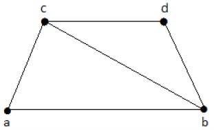
The subgraphs that can be derived from the above graph are as follows −
K1 = {b, c}
K2 = {a, b, c}
K3 = {b, c, d}
K4 = {a, d}
Here, K1, K2, and K3 have vertex covering, whereas K4 does not have any vertex covering as it does not cover the edge {bc}.
Minimal Vertex Covering
A vertex ‘K’ of graph ‘G’ is said to be minimal vertex covering if no vertex can be deleted from ‘K’.
Example
In the above graph, the subgraphs having vertex covering are as follows −
K1 = {b, c}
K2 = {a, b, c}
K3 = {b, c, d}
Here, K1 and K2 are minimal vertex coverings, whereas in K3, vertex ‘d’ can be deleted.
Minimum Vertex Covering
It is also known as the smallest minimal vertex covering. A minimal vertex covering of graph ‘G’ with minimum number of vertices is called the minimum vertex covering.
The number of vertices in a minimum vertex covering of ‘G’ is called the vertex covering number of G (α2).
Example
In the following graph, the subgraphs having vertex covering are as follows −
K1 = {b, c}
K2 = {a, b, c}
K3 = {b, c, d}
Here, K1 is a minimum vertex cover of G, as it has only two vertices. α2 = 2.
Graph Theory - Matchings
A matching graph is a subgraph of a graph where there are no edges adjacent to each other. Simply, there should not be any common vertex between any two edges.
Matching
Let ‘G’ = (V, E) be a graph. A subgraph is called a matching M(G), if each vertex of G is incident with at most one edge in M, i.e.,
deg(V) ≤ 1 ∀ V ∈ G
which means in the matching graph M(G), the vertices should have a degree of 1 or 0, where the edges should be incident from the graph G.
Notation − M(G)
Example
In a matching,
if deg(V) = 1, then (V) is said to be matched
if deg(V) = 0, then (V) is not matched.
In a matching, no two edges are adjacent. It is because if any two edges are adjacent, then the degree of the vertex which is joining those two edges will have a degree of 2 which violates the matching rule.
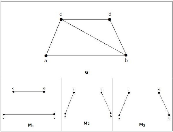
Maximal Matching
A matching M of graph ‘G’ is said to maximal if no other edges of ‘G’ can be added to M.
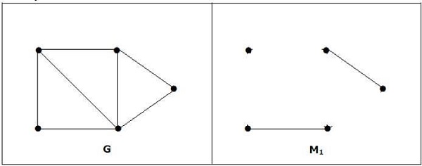
Example
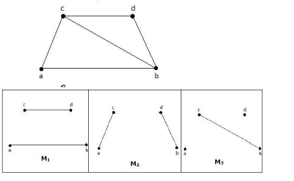
M1, M2, M3 from the above graph are the maximal matching of G.
Maximum Matching
It is also known as largest maximal matching. Maximum matching is defined as the maximal matching with maximum number of edges.
The number of edges in the maximum matching of ‘G’ is called its matching number.
Example
For a graph given in the above example, M1 and M2 are the maximum matching of ‘G’ and its matching number is 2. Hence by using the graph G, we can form only the subgraphs with only 2 edges maximum. Hence we have the matching number as two.
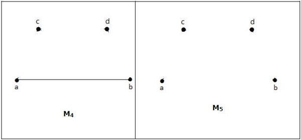
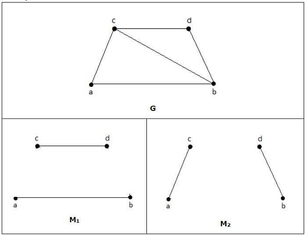
Perfect Matching
A matching (M) of graph (G) is said to be a perfect match, if every vertex of graph g (G) is incident to exactly one edge of the matching (M), i.e.,
deg(V) = 1 ∀ V
The degree of each and every vertex in the subgraph should have a degree of 1.
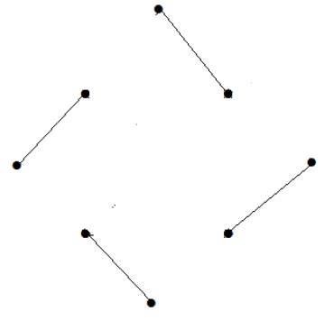
Example
In the following graphs, M1 and M2 are examples of perfect matching of G.
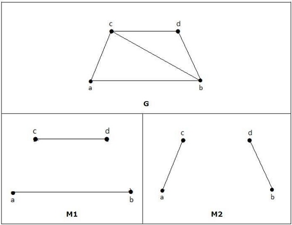
Note − Every perfect matching of graph is also a maximum matching of graph, because there is no chance of adding one more edge in a perfect matching graph.
A maximum matching of graph need not be perfect. If a graph ‘G’ has a perfect match, then the number of vertices |V(G)| is even. If it is odd, then the last vertex pairs with the other vertex, and finally there remains a single vertex which cannot be paired with any other vertex for which the degree is zero. It clearly violates the perfect matching principle.
Example
Note − The converse of the above statement need not be true. If G has even number of vertices, then M1 need not be perfect.
Example
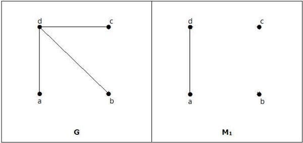
It is matching, but it is not a perfect match, even though it has even number of vertices.
Graph Theory - Independent Sets
Independent sets are represented in sets, in which
there should not be any edges adjacent to each other. There should not be any common vertex between any two edges.
there should not be any vertices adjacent to each other. There should not be any common edge between any two vertices.
Independent Line Set
Let ‘G’ = (V, E) be a graph. A subset L of E is called an independent line set of ‘G’ if no two edges in L are adjacent. Such a set is called an independent line set.
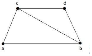
Example
Let us consider the following subsets −
L1 = {a,b}
L2 = {a,b} {c,e}
L3 = {a,d} {b,c}
In this example, the subsets L2 and L3 are clearly not the adjacent edges in the given graph. They are independent line sets. However L1 is not an independent line set, as for making an independent line set, there should be at least two edges.
Maximal Independent Line Set
An independent line set is said to be the maximal independent line set of a graph ‘G’ if no other edge of ‘G’ can be added to ‘L’.
Example
Let us consider the following subsets −
L1 = {a, b}
L2 = {{b, e}, {c, f}}
L3 = {{a, e}, {b, c}, {d, f}}
L4 = {{a, b}, {c, f}}
L2 and L3 are maximal independent line sets/maximal matching. As for only these two subsets, there is no chance of adding any other edge which is not an adjacent. Hence these two subsets are considered as the maximal independent line sets.
Maximum Independent Line Set
A maximum independent line set of ‘G’ with maximum number of edges is called a maximum independent line set of ‘G’.
Number of edges in a maximum independent line set of G (β1)
   = Line independent number of G
   = Matching number of G
Example
Let us consider the following subsets −
L1 = {a, b}
L2 = {{b, e}, {c, f}}
L3 = {{a, e}, {b, c}, {d, f}}
L4 = {{a, b}, {c, f}}
L3 is the maximum independent line set of G with maximum edges which are not the adjacent edges in graph and is denoted by β1 = 3.
Note − For any graph G with no isolated vertex,
α1 + β1 = number of vertices in a graph = |V|
Example
Line covering number of Kn/Cn/wn,
$$\alpha 1 = \lceil\frac{n}{2}\rceil\begin{cases}\frac{n}{2}\:if\:n\:is\:even \\\frac{n+1}{2}\:if\:n\:is\:odd\end{cases}$$Line independent number (Matching number) = β1 = [n/2] α1 + β1 = n.
Independent Vertex Set
Let ‘G’ = (V, E) be a graph. A subset of ‘V’ is called an independent set of ‘G’ if no two vertices in ‘S’ are adjacent.
Example
Consider the following subsets from the above graphs −
S1 = {e}

S2 = {e, f}
S3 = {a, g, c}
S4 = {e, d}
Clearly S1 is not an independent vertex set, because for getting an independent vertex set, there should be at least two vertices in the from a graph. But here it is not that case. The subsets S2, S3, and S4 are the independent vertex sets because there is no vertex that is adjacent to any one vertex from the subsets.
Maximal Independent Vertex Set
Let ‘G’ be a graph, then an independent vertex set of ‘G’ is said to be maximal if no other vertex of ‘G’ can be added to ‘S’.
Example
Consider the following subsets from the above graphs.
S1 = {e}
S2 = {e, f}
S3 = {a, g, c}
S4 = {e, d}
S2 and S3 are maximal independent vertex sets of ‘G’. In S1 and S4, we can add other vertices; but in S2 and S3, we cannot add any other vertex.
Maximum Independent Vertex Set
A maximal independent vertex set of ‘G’ with maximum number of vertices is called as the maximum independent vertex set.
Example
Consider the following subsets from the above graph −
S1 = {e}
S2 = {e, f}
S3 = {a, g, c}
S4 = {e, d}
Only S3 is the maximum independent vertex set, as it covers the highest number of vertices. The number of vertices in a maximum independent vertex set of ‘G’ is called the independent vertex number of G (β2).
Example
For the complete graph Kn,
Vertex covering number = α2 = n−1
Vertex independent number = β2 = 1
You have α2 + β2 = n
In a complete graph, each vertex is adjacent to its remaining (n − 1) vertices. Therefore, a maximum independent set of Kn contains only one vertex.
Therefore, β2=1
and α2=|v| − β2 = n-1
Note − For any graph ‘G’ = (V, E)
- α2 + β2 = |v|
- If ‘S’ is an independent vertex set of ‘G’, then (V – S) is a vertex cover of G.
Graph Theory - Coloring
Graph coloring is nothing but a simple way of labelling graph components such as vertices, edges, and regions under some constraints. In a graph, no two adjacent vertices, adjacent edges, or adjacent regions are colored with minimum number of colors. This number is called the chromatic number and the graph is called a properly colored graph.
While graph coloring, the constraints that are set on the graph are colors, order of coloring, the way of assigning color, etc. A coloring is given to a vertex or a particular region. Thus, the vertices or regions having same colors form independent sets.
Vertex Coloring
Vertex coloring is an assignment of colors to the vertices of a graph ‘G’ such that no two adjacent vertices have the same color. Simply put, no two vertices of an edge should be of the same color.
Chromatic Number
The minimum number of colors required for vertex coloring of graph ‘G’ is called as the chromatic number of G, denoted by X(G).
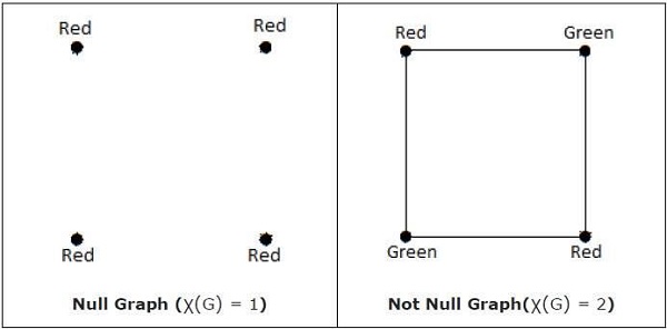
χ(G) = 1 if and only if 'G' is a null graph. If 'G' is not a null graph, then χ(G) ≥ 2.
Example
Note − A graph ‘G’ is said to be n-coverable if there is a vertex coloring that uses at most n colors, i.e., X(G) ≤ n.
Region Coloring
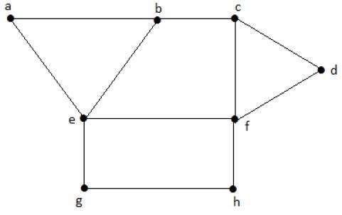
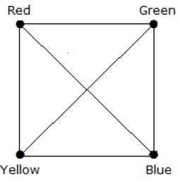
Region coloring is an assignment of colors to the regions of a planar graph such that no two adjacent regions have the same color. Two regions are said to be adjacent if they have a common edge.
Example
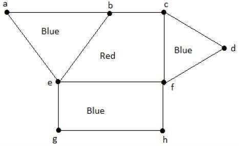
Take a look at the following graph. The regions ‘aeb’ and ‘befc’ are adjacent, as there is a common edge ‘be’ between those two regions.
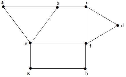
Similarly, the other regions are also coloured based on the adjacency. This graph is coloured as follows −
Example
The chromatic number of Kn is
- n
- n–1
- [n/2]
- [n/2]
Consider this example with K4.
In the complete graph, each vertex is adjacent to remaining (n – 1) vertices. Hence, each vertex requires a new color. Hence the chromatic number of Kn = n.
Applications of Graph Coloring
Graph coloring is one of the most important concepts in graph theory. It is used in many real-time applications of computer science such as −
- Clustering
- Data mining
- Image capturing
- Image segmentation
- Networking
- Resource allocation
- Processes scheduling
Graph Theory - Isomorphism
A graph can exist in different forms having the same number of vertices, edges, and also the same edge connectivity. Such graphs are called isomorphic graphs. Note that we label the graphs in this chapter mainly for the purpose of referring to them and recognizing them from one another.
Isomorphic Graphs
Two graphs G1 and G2 are said to be isomorphic if −
Their number of components (vertices and edges) are same.
Their edge connectivity is retained.
Note − In short, out of the two isomorphic graphs, one is a tweaked version of the other. An unlabelled graph also can be thought of as an isomorphic graph.
There exists a function ‘f’ from vertices of G1 to vertices of G2
   [f: V(G1) ⇒ V(G2)], such that
Case (i): f is a bijection (both one-one and onto)
Case (ii): f preserves adjacency of vertices, i.e., if the edge {U, V} ∈ G1, then the
edge {f(U), f(V)} ∈ G2, then G1 ≡ G2.
Note
If G1 ≡ G2 then −
|V(G1)| = |V(G2)|
|E(G1)| = |E(G2)|
Degree sequences of G1 and G2 are same.
If the vertices {V1, V2, .. Vk} form a cycle of length K in G1, then the vertices {f(V1), f(V2),… f(Vk)} should form a cycle of length K in G2.
All the above conditions are necessary for the graphs G1 and G2 to be isomorphic, but not sufficient to prove that the graphs are isomorphic.
(G1 ≡ G2) if and only if (G1− ≡ G2−) where G1 and G2 are simple graphs.
(G1 ≡ G2) if the adjacency matrices of G1 and G2 are same.
(G1 ≡ G2) if and only if the corresponding subgraphs of G1 and G2 (obtained by deleting some vertices in G1 and their images in graph G2) are isomorphic.
Example
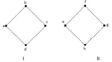
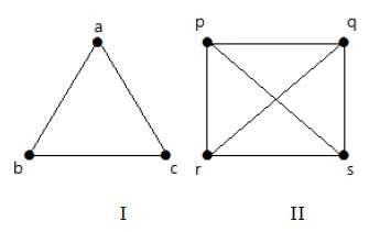
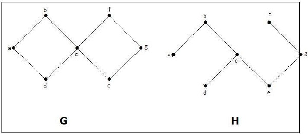
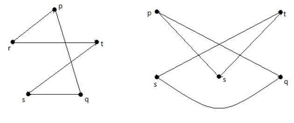
Which of the following graphs are isomorphic?
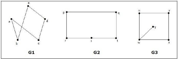
In the graph G3, vertex ‘w’ has only degree 3, whereas all the other graph vertices has degree 2. Hence G3 not isomorphic to G1 or G2.
Taking complements of G1 and G2, you have −
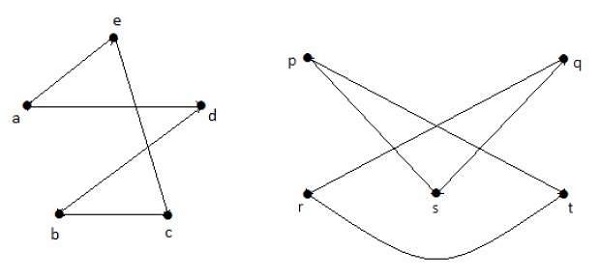
Here, (G1− ≡ G2−), hence (G1 ≡ G2).
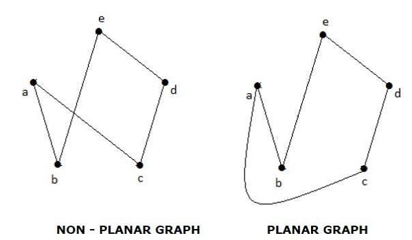
Planar Graphs
A graph ‘G’ is said to be planar if it can be drawn on a plane or a sphere so that no two edges cross each other at a non-vertex point.
Example
Regions
Every planar graph divides the plane into connected areas called regions.
Example
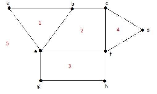
Degree of a bounded region r = deg(r) = Number of edges enclosing the regions r.
deg(1) = 3
deg(2) = 4
deg(3) = 4

deg(4) = 3
deg(5) = 8
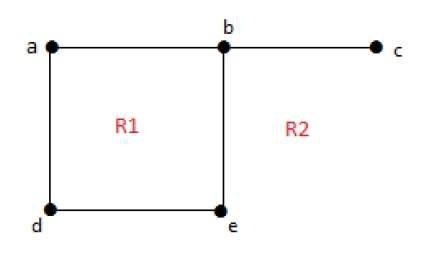
Degree of an unbounded region r = deg(r) = Number of edges enclosing the regions r.
deg(R1) = 4
deg(R2) = 6
In planar graphs, the following properties hold good −
In a planar graph with ‘n’ vertices, sum of degrees of all the vertices is −
According to Sum of Degrees of Regions/ Theorem, in a planar graph with ‘n’ regions, Sum of degrees of regions is −
Based on the above theorem, you can draw the following conclusions −
In a planar graph,
If degree of each region is K, then the sum of degrees of regions is −
If the degree of each region is at least K(≥ K), then
If the degree of each region is at most K(≤ K), then
Note − Assume that all the regions have same degree.
According to Euler’s Formulae on planar graphs,
If a graph ‘G’ is a connected planar, then
If a planar graph with ‘K’ components, then
Where, |V| is the number of vertices, |E| is the number of edges, and |R| is the number of regions.
Edge Vertex Inequality
If ‘G’ is a connected planar graph with degree of each region at least ‘K’ then,
|E| ≤ k / (k-2) {|v| - 2}
You know, |V| + |R| = |E| + 2
K.|R| ≤ 2|E|
K(|E| - |V| + 2) ≤ 2|E|
(K - 2)|E| ≤ K(|V| - 2)
|E| ≤ k / (k-2) {|v| - 2}
If ‘G’ is a simple connected planar graph, then
|E| ≤ 3|V| − 6
|R| ≤ 2|V| − 4
There exists at least one vertex V •∈ G, such that deg(V) ≤ 5.
If ‘G’ is a simple connected planar graph (with at least 2 edges) and no triangles, then
|E| ≤ {2|V| – 4}
Kuratowski’s Theorem
A graph ‘G’ is non-planar if and only if ‘G’ has a subgraph which is homeomorphic to K5 or K3,3.
Homomorphism
Two graphs G1 and G2 are said to be homomorphic, if each of these graphs can be obtained from the same graph ‘G’ by dividing some edges of G with more vertices. Take a look at the following example −
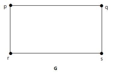
Divide the edge ‘rs’ into two edges by adding one vertex.
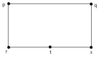
The graphs shown below are homomorphic to the first graph.
If G1 is isomorphic to G2, then G is homeomorphic to G2 but the converse need not be true.
Any graph with 4 or less vertices is planar.
Any graph with 8 or less edges is planar.
A complete graph Kn is planar if and only if n ≤ 4.
The complete bipartite graph Km, n is planar if and only if m ≤ 2 or n ≤ 2.
A simple non-planar graph with minimum number of vertices is the complete graph K5.
The simple non-planar graph with minimum number of edges is K3, 3.
Polyhedral graph
A simple connected planar graph is called a polyhedral graph if the degree of each vertex is ≥ 3, i.e., deg(V) ≥ 3 ∀ V ∈ G.
3|V| ≤ 2|E|
3|R| ≤ 2|E|
Graph Theory - Traversability
A graph is traversable if you can draw a path between all the vertices without retracing the same path. Based on this path, there are some categories like Euler’s path and Euler’s circuit which are described in this chapter.
Euler’s Path
An Euler’s path contains each edge of ‘G’ exactly once and each vertex of ‘G’ at least once. A connected graph G is said to be traversable if it contains an Euler’s path.
Example
Euler’s Path = d-c-a-b-d-e.
Euler’s Circuit
In a Euler’s path, if the starting vertex is same as its ending vertex, then it is called an Euler’s circuit.
Example
Euler’s Path = a-b-c-d-a-g-f-e-c-a.
Euler’s Circuit Theorem
A connected graph ‘G’ is traversable if and only if the number of vertices with odd degree in G is exactly 2 or 0. A connected graph G can contain an Euler’s path, but not an Euler’s circuit, if it has exactly two vertices with an odd degree.
Note − This Euler path begins with a vertex of odd degree and ends with the other vertex of odd degree.
Example
Euler’s Path − b-e-a-b-d-c-a is not an Euler’s circuit, but it is an Euler’s path. Clearly it has exactly 2 odd degree vertices.
Note − In a connected graph G, if the number of vertices with odd degree = 0, then Euler’s circuit exists.
Hamiltonian Graph
A connected graph G is said to be a Hamiltonian graph, if there exists a cycle which contains all the vertices of G.
Every cycle is a circuit but a circuit may contain multiple cycles. Such a cycle is called a Hamiltonian cycle of G.
Hamiltonian Path
A connected graph is said to be Hamiltonian if it contains each vertex of G exactly once. Such a path is called a Hamiltonian path.
Example
Hamiltonian Path− e-d-b-a-c.
Note
Euler’s circuit contains each edge of the graph exactly once.
In a Hamiltonian cycle, some edges of the graph can be skipped.
Example
Take a look at the following graph −
For the graph shown above −
Euler path exists – false
Euler circuit exists – false
Hamiltonian cycle exists – true
Hamiltonian path exists – true
G has four vertices with odd degree, hence it is not traversable. By skipping the internal edges, the graph has a Hamiltonian cycle passing through all the vertices.
Graph Theory - Examples
In this chapter, we will cover a few standard examples to demonstrate the concepts we already discussed in the earlier chapters.
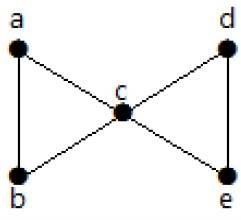
Example 1
Find the number of spanning trees in the following graph.
Solution
The number of spanning trees obtained from the above graph is 3. They are as follows −
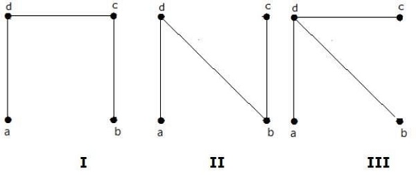
These three are the spanning trees for the given graphs. Here the graphs I and II are isomorphic to each other. Clearly, the number of non-isomorphic spanning trees is two.
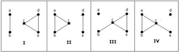
Example 2
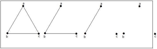
How many simple non-isomorphic graphs are possible with 3 vertices?
Solution
There are 4 non-isomorphic graphs possible with 3 vertices. They are shown below.
Example 3
Let ‘G’ be a connected planar graph with 20 vertices and the degree of each vertex is 3. Find the number of regions in the graph.
Solution
By the sum of degrees theorem,
20 Σ i=1 deg(Vi) = 2|E|
20(3) = 2|E|
|E| = 30
By Euler’s formula,
|V| + |R| = |E| + 2
20+ |R| = 30 + 2
|R| = 12
Hence, the number of regions is 12.
Example 4
What is the chromatic number of complete graph Kn?
Solution
In a complete graph, each vertex is adjacent to is remaining (n–1) vertices. Hence, each vertex requires a new color. Hence the chromatic number Kn = n.
Example 5
What is the matching number for the following graph?
Solution
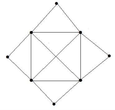
Number of vertices = 9
We can match only 8 vertices.
Matching number is 4.
Example 6
What is the line covering number of for the following graph?
Solution
Number of vertices = |V| = n = 7
Line covering number = (α1) ≥ [n/2] = 3
α1 ≥ 3
By using 3 edges, we can cover all the vertices.
Hence, the line covering number is 3.