Gensim - Documents & LDA Model

---

---

This chapter discusses the documents and LDA model in Gensim.

Finding Optimal Number of Topics for LDA

We can find the optimal number of topics for LDA by creating many LDA models with various values of topics. Among those LDAs we can pick one having highest coherence value.

Following function named coherence_values_computation() will train multiple LDA models. It will also provide the models as well as their corresponding coherence score −

def coherence_values_computation(dictionary, corpus, texts, limit, start=2, step=3):
   coherence_values = []
   model_list = []
   for num_topics in range(start, limit, step):
      model = gensim.models.wrappers.LdaMallet(
         mallet_path, corpus=corpus, num_topics=num_topics, id2word=id2word
      )
      model_list.append(model)
   coherencemodel = CoherenceModel(
      model=model, texts=texts, dictionary=dictionary, coherence='c_v'
   )
   coherence_values.append(coherencemodel.get_coherence())
return model_list, coherence_values

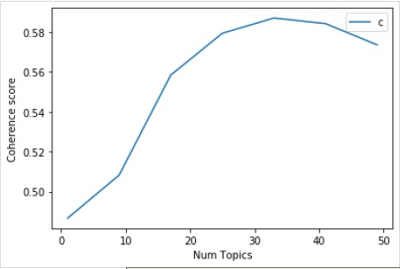
Now with the help of following code, we can get the optimal number of topics which we can show with the help of a graph as well −

model_list, coherence_values = coherence_values_computation (
   dictionary=id2word, corpus=corpus, texts=data_lemmatized, 
   start=1, limit=50, step=8
)
limit=50; start=1; step=8;
x = range(start, limit, step)
plt.plot(x, coherence_values)
plt.xlabel("Num Topics")
plt.ylabel("Coherence score")
plt.legend(("coherence_values"), loc='best')
plt.show()

Output

Next, we can also print the coherence values for various topics as follows −

for m, cv in zip(x, coherence_values):
   print("Num Topics =", m, " is having Coherence Value of", round(cv, 4))

Output

Num Topics = 1 is having Coherence Value of 0.4866
Num Topics = 9 is having Coherence Value of 0.5083
Num Topics = 17 is having Coherence Value of 0.5584
Num Topics = 25 is having Coherence Value of 0.5793
Num Topics = 33 is having Coherence Value of 0.587
Num Topics = 41 is having Coherence Value of 0.5842
Num Topics = 49 is having Coherence Value of 0.5735

Now, the question arises which model should we pick now? One of the good practices is to pick the model, that is giving highest coherence value before flattering out. So that’s why, we will be choosing the model with 25 topics which is at number 4 in the above list.

optimal_model = model_list[3]
model_topics = optimal_model.show_topics(formatted=False)
pprint(optimal_model.print_topics(num_words=10))

[
   (0,
   '0.018*"power" + 0.011*"high" + 0.010*"ground" + 0.009*"current" + '
   '0.008*"low" + 0.008*"wire" + 0.007*"water" + 0.007*"work" + 0.007*"design" '
   '+ 0.007*"light"'),
   (1,
   '0.036*"game" + 0.029*"team" + 0.029*"year" + 0.028*"play" + 0.020*"player" '
   '+ 0.019*"win" + 0.018*"good" + 0.013*"season" + 0.012*"run" + 0.011*"hit"'),
   (2,
   '0.020*"image" + 0.019*"information" + 0.017*"include" + 0.017*"mail" + '
   '0.016*"send" + 0.015*"list" + 0.013*"post" + 0.012*"address" + '
   '0.012*"internet" + 0.012*"system"'),
   (3,
   '0.986*"ax" + 0.002*"_" + 0.001*"tm" + 0.000*"part" + 0.000*"biz" + '
   '0.000*"mb" + 0.000*"mbs" + 0.000*"pne" + 0.000*"end" + 0.000*"di"'),
   (4,
   '0.020*"make" + 0.014*"work" + 0.013*"money" + 0.013*"year" + 0.012*"people" '
   '+ 0.011*"job" + 0.010*"group" + 0.009*"government" + 0.008*"support" + '
   '0.008*"question"'),
   (5,
   '0.011*"study" + 0.011*"drug" + 0.009*"science" + 0.008*"food" + '
   '0.008*"problem" + 0.008*"result" + 0.008*"effect" + 0.007*"doctor" + '
   '0.007*"research" + 0.007*"patient"'),
   (6,
   '0.024*"gun" + 0.024*"law" + 0.019*"state" + 0.015*"case" + 0.013*"people" + '
   '0.010*"crime" + 0.010*"weapon" + 0.010*"person" + 0.008*"firearm" + '
   '0.008*"police"'),
   (7,
   '0.012*"word" + 0.011*"question" + 0.011*"exist" + 0.011*"true" + '
   '0.010*"religion" + 0.010*"claim" + 0.008*"argument" + 0.008*"truth" + '
   '0.008*"life" + 0.008*"faith"'),
   (8,
   '0.077*"time" + 0.029*"day" + 0.029*"call" + 0.025*"back" + 0.021*"work" + '
   '0.019*"long" + 0.015*"end" + 0.015*"give" + 0.014*"year" + 0.014*"week"'),
   (9,
   '0.048*"thing" + 0.041*"make" + 0.038*"good" + 0.037*"people" + '
   '0.028*"write" + 0.019*"bad" + 0.019*"point" + 0.018*"read" + 0.018*"post" + '
   '0.016*"idea"'),
   (10,
   '0.022*"book" + 0.020*"_" + 0.013*"man" + 0.012*"people" + 0.011*"write" + '
   '0.011*"find" + 0.010*"history" + 0.010*"armenian" + 0.009*"turkish" + '
   '0.009*"number"'),
   (11,
   '0.064*"line" + 0.030*"buy" + 0.028*"organization" + 0.025*"price" + '
   '0.025*"sell" + 0.023*"good" + 0.021*"host" + 0.018*"sale" + 0.017*"mail" + '
   '0.016*"cost"'),
   (12,
   '0.041*"car" + 0.015*"bike" + 0.011*"ride" + 0.010*"engine" + 0.009*"drive" '
   '+ 0.008*"side" + 0.008*"article" + 0.007*"turn" + 0.007*"front" + '
   '0.007*"speed"'),
   (13,
   '0.018*"people" + 0.011*"attack" + 0.011*"state" + 0.011*"israeli" + '
   '0.010*"war" + 0.010*"country" + 0.010*"government" + 0.009*"live" + '
   '0.009*"give" + 0.009*"land"'),
   (14,
   '0.037*"file" + 0.026*"line" + 0.021*"read" + 0.019*"follow" + '
   '0.018*"number" + 0.015*"program" + 0.014*"write" + 0.012*"entry" + '
   '0.012*"give" + 0.011*"check"'),
   (15,
   '0.196*"write" + 0.172*"line" + 0.165*"article" + 0.117*"organization" + '
   '0.086*"host" + 0.030*"reply" + 0.010*"university" + 0.008*"hear" + '
   '0.007*"post" + 0.007*"news"'),
   (16,
   '0.021*"people" + 0.014*"happen" + 0.014*"child" + 0.012*"kill" + '
   '0.011*"start" + 0.011*"live" + 0.010*"fire" + 0.010*"leave" + 0.009*"hear" '
   '+ 0.009*"home"'),
   (17,
   '0.038*"key" + 0.018*"system" + 0.015*"space" + 0.015*"technology" + '
   '0.014*"encryption" + 0.010*"chip" + 0.010*"bit" + 0.009*"launch" + '
   '0.009*"public" + 0.009*"government"'),
   (18,
   '0.035*"drive" + 0.031*"system" + 0.027*"problem" + 0.027*"card" + '
   '0.020*"driver" + 0.017*"bit" + 0.017*"work" + 0.016*"disk" + '
   '0.014*"monitor" + 0.014*"machine"'),
   (19,
   '0.031*"window" + 0.020*"run" + 0.018*"color" + 0.018*"program" + '
   '0.017*"application" + 0.016*"display" + 0.015*"set" + 0.015*"version" + '
   '0.012*"screen" + 0.012*"problem"')
]

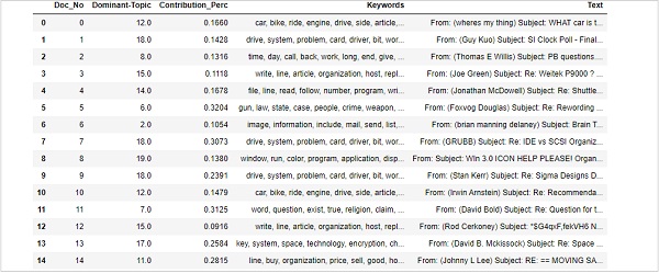
Finding dominant topics in sentences

Finding dominant topics in sentences is one of the most useful practical applications of topic modeling. It determines what topic a given document is about. Here, we will find that topic number which has the highest percentage contribution in that particular document. In order to aggregate the information in a table, we will be creating a function named dominant_topics() −

def dominant_topics(ldamodel=lda_model, corpus=corpus, texts=data):
   sent_topics_df = pd.DataFrame()

Next, we will get the main topics in every document −

for i, row in enumerate(ldamodel[corpus]):
   row = sorted(row, key=lambda x: (x[1]), reverse=True)

Next, we will get the Dominant topic, Perc Contribution and Keywords for every document −

for j, (topic_num, prop_topic) in enumerate(row):
   if j == 0: # => dominant topic
      wp = ldamodel.show_topic(topic_num)
      topic_keywords = ", ".join([word for word, prop in wp])
sent_topics_df = sent_topics_df.append(
   pd.Series([int(topic_num), round(prop_topic,4), topic_keywords]), ignore_index=True
)
   else:
      break
sent_topics_df.columns = ['Dominant_Topic', 'Perc_Contribution', 'Topic_Keywords']

With the help of following code, we will add the original text to the end of the output −

contents = pd.Series(texts)
   sent_topics_df = pd.concat([sent_topics_df, contents], axis=1)
   return(sent_topics_df)
df_topic_sents_keywords = dominant_topics(
   ldamodel=optimal_model, corpus=corpus, texts=data
)

Now, do the formatting of topics in the sentences as follows −

df_dominant_topic = df_topic_sents_keywords.reset_index()
df_dominant_topic.columns = [
   'Document_No', 'Dominant_Topic', 'Topic_Perc_Contrib', 'Keywords', 'Text'
]

Finally, we can show the dominant topics as follows −

df_dominant_topic.head(15)

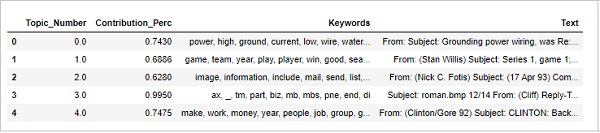
Finding Most Representative Document

In order to understand more about the topic, we can also find the documents, a given topic has contributed to the most. We can infer that topic by reading that particular document(s).

sent_topics_sorteddf_mallet = pd.DataFrame()
sent_topics_outdf_grpd = df_topic_sents_keywords.groupby('Dominant_Topic')
for i, grp in sent_topics_outdf_grpd:
   sent_topics_sorteddf_mallet = pd.concat([sent_topics_sorteddf_mallet,
grp.sort_values(['Perc_Contribution'], ascending=[0]).head(1)], axis=0)
sent_topics_sorteddf_mallet.reset_index(drop=True, inplace=True)
sent_topics_sorteddf_mallet.columns = [
   'Topic_Number', "Contribution_Perc", "Keywords", "Text"
]
sent_topics_sorteddf_mallet.head()

Output

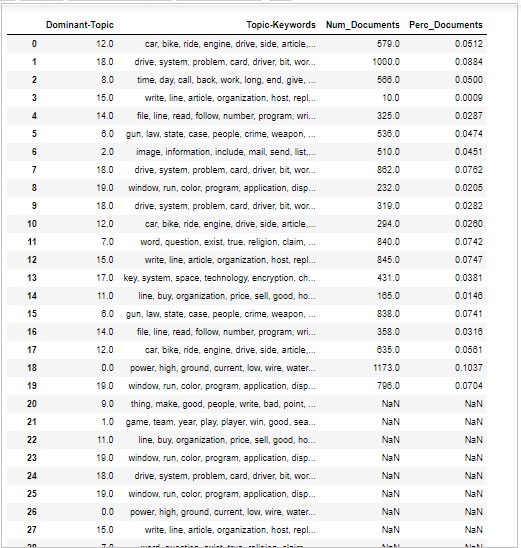
Volume & Distribution of Topics

Sometimes we also want to judge how widely the topic is discussed in documents. For this we need to understand the volume and distribution of topics across the documents.

First calculate the number of documents for every Topic as follows −

topic_counts = df_topic_sents_keywords['Dominant_Topic'].value_counts()

Next, calculate the percentage of Documents for every Topic as follows −;

topic_contribution = round(topic_counts/topic_counts.sum(), 4)

Now find the topic Number and Keywords as follows −

topic_num_keywords = df_topic_sents_keywords[['Dominant_Topic', 'Topic_Keywords']]

Now, concatenate then Column wise as follows −

df_dominant_topics = pd.concat(
   [topic_num_keywords, topic_counts, topic_contribution], axis=1
)

Next, we will change the Column names as follows −

df_dominant_topics.columns = [
   'Dominant-Topic', 'Topic-Keywords', 'Num_Documents', 'Perc_Documents'
]
df_dominant_topics

Output