Excel Pivot Tables - Filtering Data

You might have to do in-depth analysis on a subset of your PivotTable data. This might be because you have large data and your focus is required on a smaller portion of the data or irrespective of the size of the data, your focus is required on certain specific data. You can filter the data in the PivotTable based on a subset of the values of one or more fields. There are several ways to do that as follows −

Filtering using Slicers.
Filtering using Report Filters.
Filtering data manually.
Filtering using Label Filters.
Filtering using Value Filters.
Filtering using Date Filters.
Filtering using Top 10 Filter.
Filtering using Timeline.

You will learn filtering data using Slicers in the next chapter. You will understand filtering by the other methods mentioned above in this chapter.

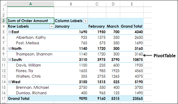
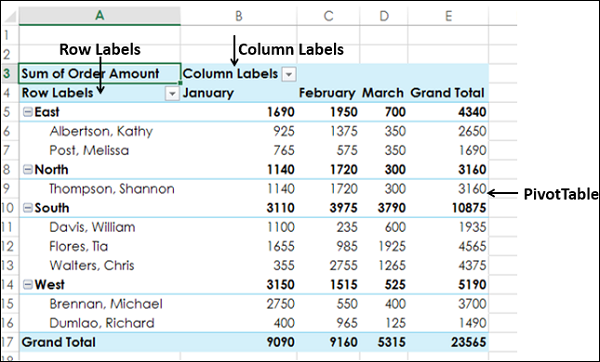
Consider the following PivotTable wherein you have the summarized sales data region wise, salesperson wise and month wise.

Report Filters

You can assign a Filter to one of the fields so that you can dynamically change the PivotTable based on the values of that field.

Drag Region from Rows to Filters in the PivotTable Areas.

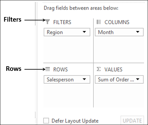
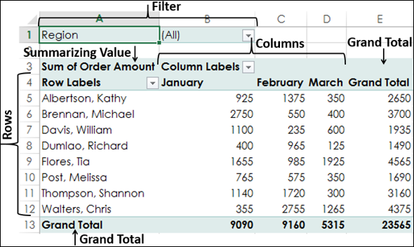
The Filter with the label as Region appears above the PivotTable (in case you do not have empty rows above your PivotTable, PivotTable gets pushed down to make space for the Filter.

You will observe that

Salesperson values appear in rows.
Month values appear in columns.
Region Filter appears on the top with default selected as ALL.
Summarizing value is Sum of Order Amount.
- Sum of Order Amount Salesperson-wise appears in the column Grand Total.
- Sum of Order Amount Month-wise appears in the row Grand Total.
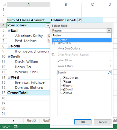
Click on the arrow in the box to the right of the Filter Region.

A drop-down list with the values of the field Region appears. Check the box Select Multiple Items.

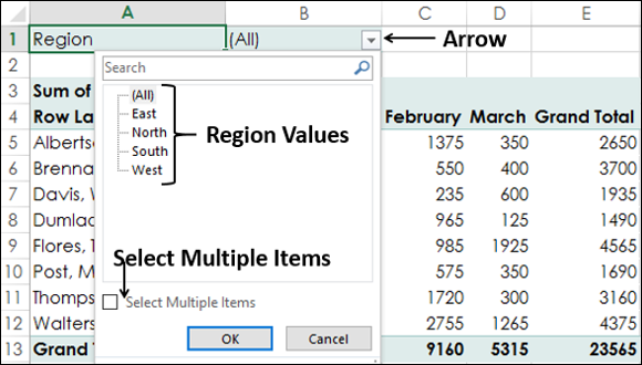
By default, all the boxes are checked. Uncheck the box (All). All the boxes will be unchecked.

Then check the boxes - South and West and click OK.

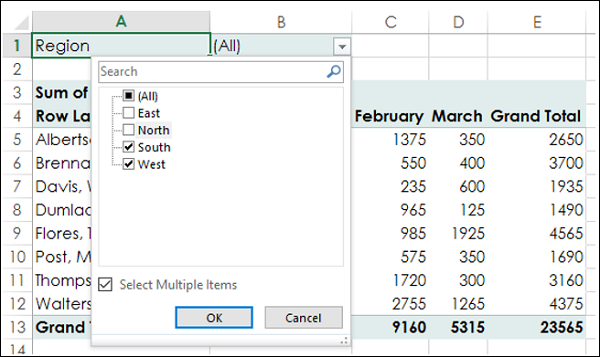
The data pertaining to South and West regions only will get summarized.

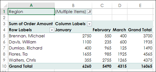
In the cell next to the Filter Region - (Multiple Items) is displayed, indicating that you have selected more than one item. However, how many items and / or which items is not known from the report that is displayed. In such a case, using Slicers is a better option for filtering.

Manual Filtering

You can also filter the PivotTable by picking the values of a field manually. You can do this by clicking on the arrow Down Arrow in the Row Labels or Column Labels cell.

Suppose you want to analyze only February data. You need to filter the values by the field Month. As you can observe, Month is part of Column Labels.

Click on the arrow Down Arrow in the Column Labels cell.

As you can observe, there is a Search box in the dropdown list and below the box, you have the list of the values of the selected field, i.e. Month. The boxes of all the values are checked, showing that all the values of that field are selected.

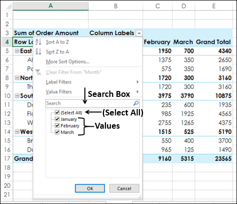
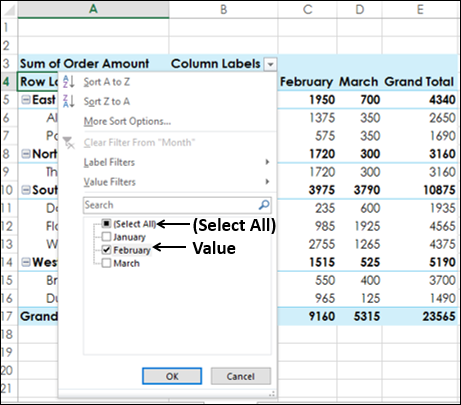
Uncheck the (Select All) box at the top of the list of values.
Check the boxes of the values you want to show in your PivotTable, in this case February and click OK.

The PivotTable displays only those values that are related to the selected Month field value – February. You can observe that the filtering arrow changes to the icon Filter Search to indicate that a filter is applied. Place the cursor on the icon.

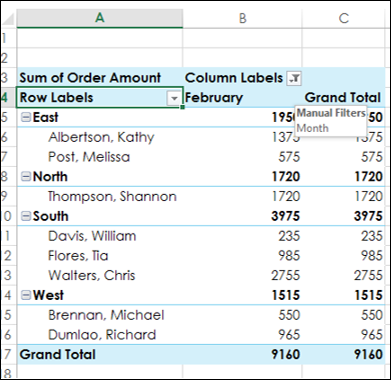
You can observe that is displayed indicating that the Manual Filter is applied on the field- Month.

If you want to change the filter selection value, do the following −

Click the icon.
Check / uncheck the boxes of the values.

If all the values of the field are not visible in the list, drag the handle in the bottom-right corner of the dropdown to enlarge it. Alternatively, if you know the value, type it in the Search box.

Suppose you want to apply another filter on the above filtered PivotTable. For example, you want to display the data of that of Walters, Chris for the month February. You need to refine your filtering by adding another filter for the field Salesperson. As you can observe, Salesperson is part of Row Labels.

Click on the arrow in the Row Labels cell.

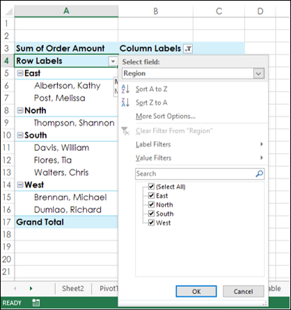
The list of the values of the field – Region is displayed. This is because, Region is at outer level of Salesperson in the nesting order. You also have an additional option – Select Field. Click on the Select Field box.

Click Salesperson from the dropdown list. The list of the values of the field – Salesperson will be displayed.
Uncheck (Select All) and check Walters, Chris.
Click OK.

The PivotTable displays only those values that are related to the selected Month field value – February and Salesperson field value - Walters, Chris.

The filtering arrow for Row Labels also changes to the icon Filter Search to indicate that a filter is applied. Place the cursor on the icon on either Row Labels or Column Labels.

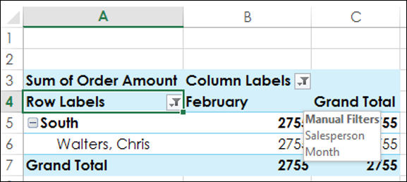
A text box is displayed indicating that the Manual Filter is applied on the fields – Month, and Salesperson.

You can thus filter the PivotTable manually based on any number of fields and on any number of values.

Filtering by Text

If you have fields that contain text, you can filter the PivotTable by Text, provided the corresponding field label is text-based. For example, consider the following Employee data.

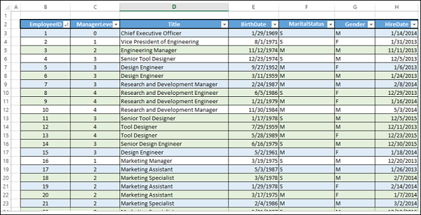
The data has the details of the employees – EmployeeID, Title, BirthDate, MaritalStatus, Gender and HireDate. Additionally, the data also has the manager level of the employee (levels 0 – 4).

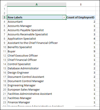
Suppose you have to do some analysis on the number of employees reporting to a given employee by title. You can create a PivotTable as given below.

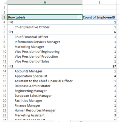
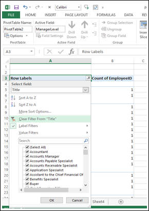
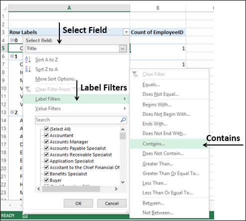
You might want to know how many employees with ‘Manager’ in their title have employees reporting to them. As the Label Title is text-based, you can apply the Label Filter on the Title field as follows −

Click on the arrow in the Row Labels cell.
Select Title in the Select Field box from the drop down list.
Click on Label Filters.
Click on Contains in the second dropdown list.

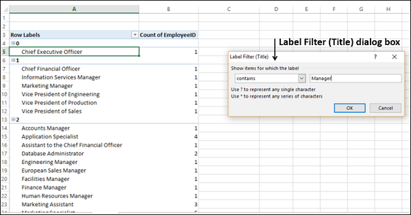
Label Filter (Title) dialog box appears. Type Manager in the box next to Contains. Click OK.

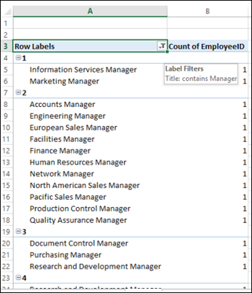
The PivotTable will be filtered to the Title values containing ‘Manager’.

Click the icon.

You can see that 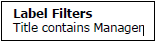Filter Button is displayed indicating the following −

The Label Filter is applied on the field – Title, and
What the applied Label Filter is.

Filtering by Values

You might want to know the titles of the employees who have more than 25 employees reporting to them. For this, you can apply the Value Filter on the Title field as follows −

Click on the arrow in the Row Labels cell.
Select Title in the Select Field box from the drop down list.
Click on Value Filters.
Select Greater than or equal to from the second dropdown list.

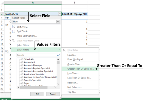
The Value Filter (Title) dialog box appears. Type 25 in the right side box.

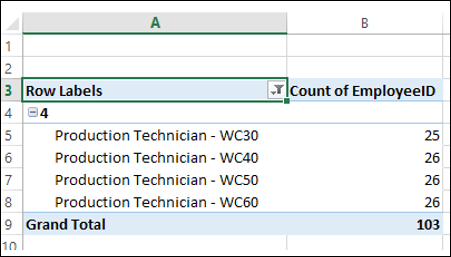
The PivotTable will be filtered to display the employee titles who have more than 25 employees reporting to them.

Filtering by Dates

You might want to display the data of all the employees who were hired in the fiscal year 2015-15. You can use Data Filters for the same as follows −

Include the HireDate field in the PivotTable. Now, you do not require manager data and so remove ManagerLevel field from the PivotTable.

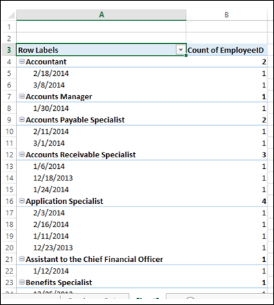
Now that you have a Date field in the PivotTable, you can use Date Filters.

Click the arrow in the Row Labels cell.
Select HireDate in the Select Field box from the drop down list.
Click Date Filters.
Seelct Between from the second dropdown list.

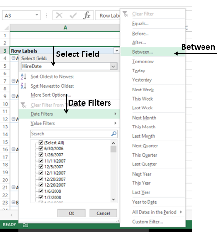
The Date Filter (HireDate) dialog box appears. Type 4/1/2014 and 3/31/2015 in the two Date boxes. Click OK.

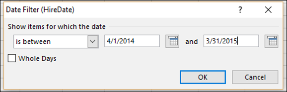
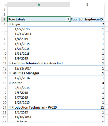
The PivotTable will be filtered to display only the data with HireDate between 1^st April 2014 and 31^st March 2015.

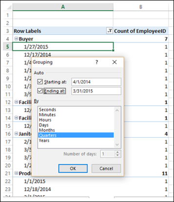
You can group the dates into Quarters as follows −

Right click on any of the dates. The Grouping dialog box appears.
Type 4/1/2014 in the box Starting at. Check the box.
Type 3/31/2015 in the box Ending at. Check the box.
Click Quarters in the box under By.

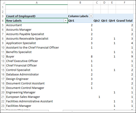
The dates will be grouped into quarters in the PivotTable. You can make the table look compact by dragging the field HireDate from ROWS area to COLUMNS area.

You will be able to know how many employees were hired during the fiscal year, quarter wise.

Filtering Using Top 10 Filter

You can use the Top 10 Filter to display the top few or bottom few values of a field in the PivotTable.

Click the arrow in the Row Labels cell.
Click Value Filters.
Click Top 10 in the second dropdown list.

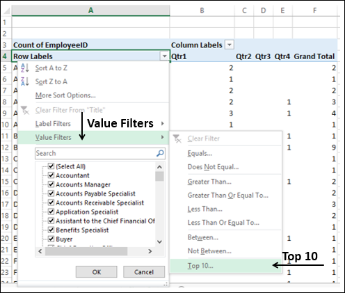
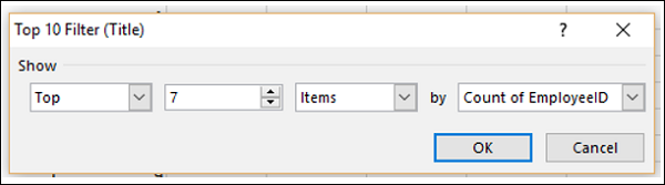
Top 10 Filter (Title) dialog box appears.

In the first box, click on Top (You can choose Bottom also).
In the second box, enter a number, say, 7.
In the third box, you have three options by which you can filter.
- Click on Items to filter by number of items.
- Click on Percent to filter by percentage.
- Click on Sum to filter by sum.
As you have count of EmployeeID, click Items.
In the fourth box, click on the field Count of EmployeeID.
Click OK.

The top seven values by count of EmployeeID will be displayed in the PivotTable.

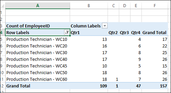
As you can observe, the highest number of hires in the fiscal year is that of Production Technicians and a predominant number of these are in Qtr1.

Filtering Using Timeline

If your PivotTable has a date field, you can filter the PivotTable using Timeline.

Create a PivotTable from the Employee Data that you used earlier and add the data to the Data Model in the Create PivotTable dialog box.

Drag the field Title to ROWS area.
Drag the field EmployeeID to ∑ VALUES area and choose Count for calculation.

Click on the PivotTable.
Click the INSERT tab.
Click Timeline in the Filters group. The Insert Timelines dialog box appears.

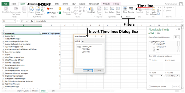
Check the box HireDate.
Click OK. The Timeline appears in the worksheet.
Timeline Tools appear on the Ribbon.

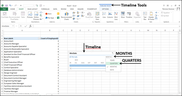
As you can observe, All Periods – in Months are displayed on the Timeline.

Click on the arrow next to - MONTHS.
Select QUARTERS from the drop-down list. The The Timeline display changes to All Periods – in Quarters.

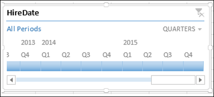
Click on 2014 Q1.
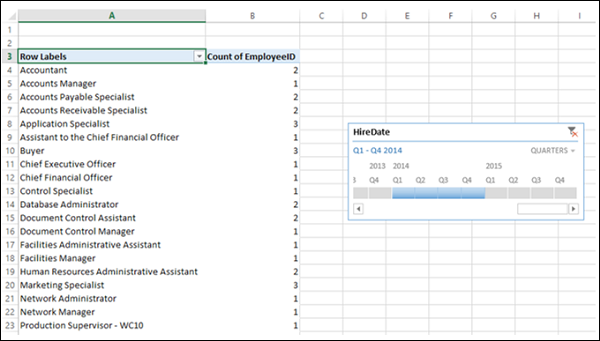
Keep the Shift key pressed and drag to 2014 Q4. The Timeline Period is selected to Q1 – Q4 2014.
PivotTable is filtered to this Timeline Period.

Clearing the Filters

You might have to clear the filters you have set from time to time to switch across different combinations and projections of your data. You can do this in several ways as follows −

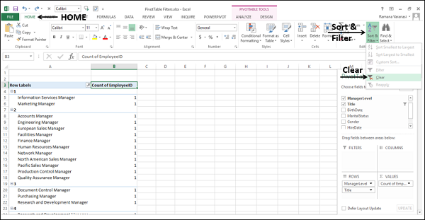
Clearing all the filters in a PivotTable

You can clear all the filters set in a PivotTable at one go as follows −

Click the HOME tab on the Ribbon.
Click Sort & Filter in the Editing group.
Select Clear from the dropdown list.

Clearing a Label, Date or Value Filter

To clear a Label, Date, or Value Filter do the following −

Click on the icon in the Row Labels or Column Labels.
Click on the <field name> from which you want to clear the filter in the Select Field box in the dropdown list.
Click on Clear Filter From <Filed Name> that appears in the dropdown list.
Click OK. The specific filter will be cleared.