- Excel Pivot Tables Tutorial
- Excel Pivot Tables - Home
- Excel Pivot Tables - Overview
- Excel Pivot Tables - Creation
- Excel Pivot Tables - Fields
- Excel Pivot Tables - Areas
- Excel Pivot Tables - Exploring Data
- Excel Pivot Tables - Sorting Data
- Excel Pivot Tables - Filtering Data
- Filtering data using Slicers
- Excel Pivot Tables - Nesting
- Excel Pivot Tables - Tools
- Summarizing Values
- Excel Pivot Tables - Updating Data
- Excel Pivot Tables - Reports
- Excel Pivot Tables Useful Resources
- Excel Pivot Tables - Quick Guide
- Excel Pivot Tables - Resources
- Excel Pivot Tables - Discussion
Excel Pivot Tables - Fields
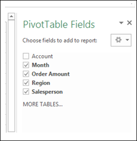
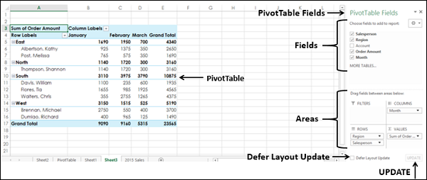
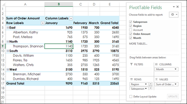
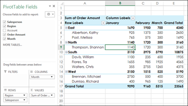
PivotTable Fields is a Task Pane associated with a PivotTable. The PivotTable Fields Task Pane comprises of Fields and Areas. By default, the Task Pane appears at the right side of the window with Fields displayed above Areas.
Fields represent the columns in your data – range or Excel table, and will have check boxes. The selected fields are displayed in the report. Areas represent the layout of the report and the calculations included in the report.
At the bottom of the Task Pane, you will find an option – Defer Layout Update with an UPDATE button next to it.
By default, this is not selected and whatever changes you make in the selection of fields or in the layout options are reflected in the PivotTable instantly.
If you select this, the changes in your selections are not updated until you click on the UPDATE button.
In this chapter, you will understand the details about Fields. In the next chapter, you will understand the details about Areas.
PivotTable Fields Task Pane
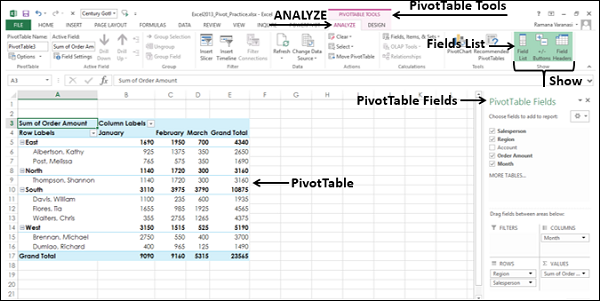
You can find the PivotTable Fields Task Pane on the worksheet where you have a PivotTable. To view the PivotTable Fields Task Pane, click the PivotTable. In case the PivotTable Fields Task Pane is not displayed, check the Ribbon for the following −
- Click the ANALYZE tab under PIVOTTABLE TOOLS on the Ribbon.
- Check if Fields List is selected (i.e. highlighted) in the Show group.
- If Fields List is not selected, then click it.
The PivotTable Fields Task Pane will be displayed on the right side of the window, with the title – PivotTable Fields.
Moving PivotTable Fields Task Pane
On the right of the title PivotTable Fields of the PivotTable Task Pane, you will find the button ![]() . This represents Task Pane Options. Click the button
. This represents Task Pane Options. Click the button ![]() . The Task Pane Options- Move, Size and Close appear in the dropdown list.
. The Task Pane Options- Move, Size and Close appear in the dropdown list.
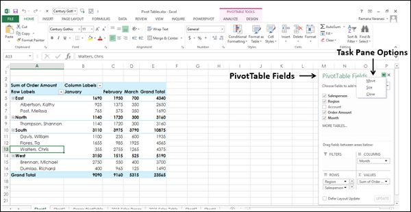
You can move the PivotTables Task Pane to anywhere you want in the window as follows −
Click Move in the dropdown list. The
 button appears on the Task Pane.
Click the
icon and drag the pane to a position where you want to place it. You can place the Task Pane next to the PivotTable as given below.
You can place the Task Pane on the left side of the window as given below.
Resizing PivotTable Fields Task Pane
You can resize the PivotTables Task Pane – i.e. increase / decrease the Task Pane length and/or width as follows −
Click on Task Pane Options −
 that is on the right side of the title - PivotTable Fields.
Click on Size in the dropdown list.
Use the symbol ⇔ to increase / decrease the width of the Task Pane.
Use the symbol ⇕ to increase / decrease the width of the Task Pane.
In the ∑ VALUES area, to make Sum of Order Amount visible completely, you can resize the Task Pane as given below.
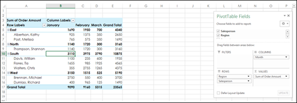
PivotTable Fields
The PivotTable Fields list comprises of all the tables that are associated with your workbook and the corresponding fields. It is by selecting the fields in the PivotTable fields list, you will create the PivotTable.
The tables and the corresponding fields with check boxes, reflect your PivotTable data. As you can check / uncheck the fields randomly, you can quickly change the PivotTable, highlighting the summarized data that you want to report or present.
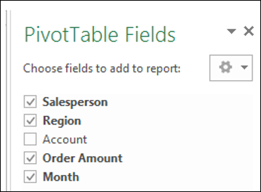
As you can observe, if there is only one table, the table name will not be displayed in the PivotTable Fields list. Only the fields will be displayed with check boxes.
Above the fields list, you will find the action Choose fields to add to report. To the right, you will find the button −  that represents Tools.
- Click on the Tools button.
In the dropdown list, you will find the following −
Five different layout options for Fields and Areas.
Two options for Sort order of the fields in the Fields list −
Sort A to Z.
Sort in Data Source Order.
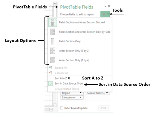
As you can observe in the above Fields list, the Sort order is by default – i.e. in Data Source Order. This means, it is the order in which the columns in your data table appear.
Normally, you can retain the default order. However, at times, you might encounter many fields in a table and might not be acquainted with them. In such a case, you can sort the fields in alphabetical order by clicking on – Sort A to Z in the dropdown list of Tools. Then, the PivotTable Fields list looks as follows −