- Excel Pivot Tables Tutorial
- Excel Pivot Tables - Home
- Excel Pivot Tables - Overview
- Excel Pivot Tables - Creation
- Excel Pivot Tables - Fields
- Excel Pivot Tables - Areas
- Excel Pivot Tables - Exploring Data
- Excel Pivot Tables - Sorting Data
- Excel Pivot Tables - Filtering Data
- Filtering data using Slicers
- Excel Pivot Tables - Nesting
- Excel Pivot Tables - Tools
- Summarizing Values
- Excel Pivot Tables - Updating Data
- Excel Pivot Tables - Reports
- Excel Pivot Tables Useful Resources
- Excel Pivot Tables - Quick Guide
- Excel Pivot Tables - Resources
- Excel Pivot Tables - Discussion
Excel Pivot Tables - Creation
You can create a PivotTable either from a range of data or from an Excel table. In both the cases, the first row of the data should contain the headers for the columns.
If you are sure of the fields to be included in the PivotTable and the layout you want to have, you can start with an empty PivotTable and construct the PivotTable.
In case you are not sure which PivotTable layout is best suitable for your data, you can make use of Recommended PivotTables command of Excel to view the PivotTables customized to your data and choose the one you like.
Creating a PivotTable from a Data Range
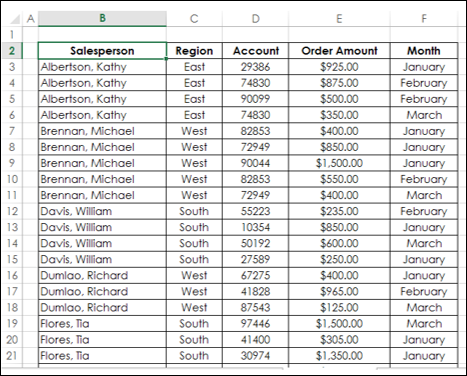
Consider the following data range that contains the sales data for each Salesperson, in each Region and in the months of January, February and March −
To create a PivotTable from this data range, do the following −
Ensure that the first row has headers. You need headers because they will be the field names in your PivotTable.
Name the data range as SalesData_Range.
Click on the data range – SalesData_Range.
Click the INSERT tab on the Ribbon.
Click PivotTable in the Tables group. The Create PivotTable dialog box appears.
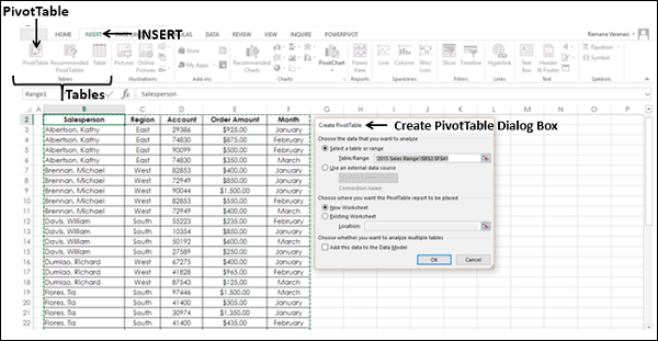
In Create PivotTable dialog box, under Choose the data that you want to analyze, you can either select a Table or Range from the current workbook or use an external data source.
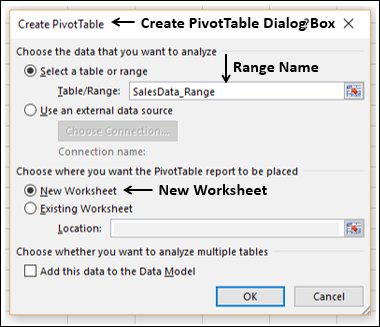
As you are creating a PivotTable from a data range, select the following from the dialog box −
Select Select a table or range.
In the Table/Range box, type the range name – SalesData_Range.
Select New Worksheet under Choose where you want the PivotTable report to be placed and click OK.
You can choose to analyze multiple tables, by adding this data range to Data Model. You can learn how to analyze multiple tables, use of Data Model and how to use an external data source to create a PivotTable in the tutorial Excel PowerPivot.
A new worksheet is inserted into your workbook. The new worksheet contains an empty PivotTable. Name the worksheet – Range-PivotTable.
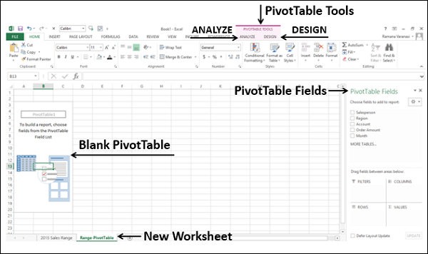
As you can observe, the PivotTable Fields list appears on the right side of the worksheet, containing the header names of the columns in the data range. Further, on the Ribbon, PivotTable Tools – ANALYZE and DESIGN appear.
Adding Fields to the PivotTable
You will understand in detail about PivotTable Fields and Areas in the later chapters in this tutorial. For now, observe the steps to add fields to the PivotTable.
Suppose you want to summarize the order amount salesperson-wise for the months January, February, and March. You can do it in few simple steps as follows −
Click on the field Salesperson in the PivotTable Fields list and drag it to the ROWS area.
Click the field Month in the PivotTable Fields list and drag that also to ROWS area.
Click on Order Amount and drag it to ∑ VALUES area.
Your first PivotTable is ready as shown below
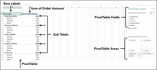
Observe that two columns appear in the PivotTable, one containing the Row Labels that you selected, i.e. Salesperson and Month and a second one containing Sum of Order Amount. In addition to Sum of Order Amount month wise for each Salesperson, you will also get subtotals representing the total sales by that person. If you scroll down the worksheet, you will find the last row as Grand Total representing total sales.
You will learn more about producing PivotTables as per the need as you progress through this tutorial.
Creating a PivotTable from a Table
Consider the following Excel table that contains the same sales data as in the previous section −
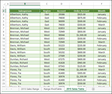
An Excel table will inherently have a name and the columns will have headers, which is a requirement to create a PivotTable. Suppose the table name is SalesData_Table.
To create a PivotTable from this Excel table, do the following −
Click on the table – SalesData_Table.
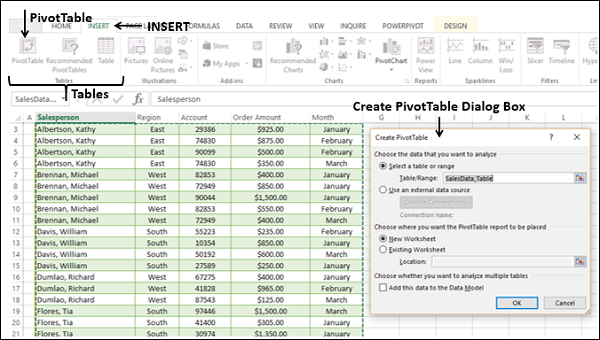
Click the INSERT tab on the Ribbon.
Click PivotTable in the Tables group. The Create PivotTable dialog box appears.
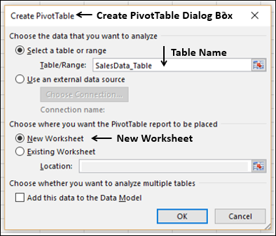
Click Select a table or range.
In the Table/Range box, type the table name – SalesData_Table.
Select New Worksheet under Choose where you want the PivotTable report to be placed. Click OK.
A new worksheet is inserted into your workbook. The new worksheet contains an empty PivotTable. Name the worksheet – Table-PivotTable. The worksheet – Table-PivotTable looks similar to the one you have got in the data range case in the earlier section.
You can add fields to the PivotTable as you have seen in the section – Adding Fields to the PivotTable, earlier in this chapter.
Creating a PivotTable with Recommended PivotTables
In case you are not familiar with Excel PivotTables or if you do not know which fields would result in a meaningful report, you can use the Recommended PivotTables command in Excel. Recommended PivotTables gives you all the possible reports with your data along with the associated layout. In other words, the options displayed will be the PivotTables that are customized to your data.
To create a PivotTable from the Excel table SalesData-Table using Recommended PivotTables, proceed as follows −
Click on the table SalesData-Table.
Click the INSERT tab.
Click Recommended PivotTables in the Tables group. The Recommended PivotTables Dialog Box appears.
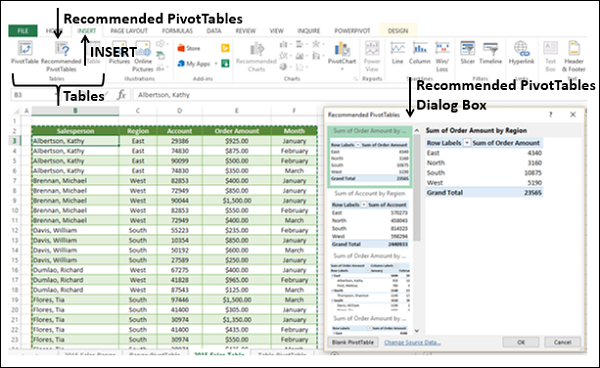
In the Recommended PivotTables dialog box, the possible customized PivotTables that suit your data will be displayed.
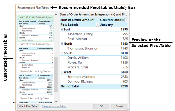
Click on each of the PivotTable options to see the preview on the right side.
Click on the PivotTable - Sum of Order Amount by Salesperson and Month and click OK.
You will be get the preview on the right side.
The selected PivotTable appears on a new worksheet in your workbook.
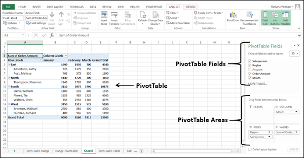
You can see that the PivotTable Fields - Salesperson, Region, Order Amount and Month got selected. Of these, Region and Salesperson are in ROWS area, Month is in COLUMNS area, and Sum of Order Amount is in ∑ VALUES area.
The PivotTable summarized the data Region-wise, Salesperson-wise and Month-wise. The subtotals are displayed for each Region, each Salesperson, and each Month.