Excel Charts - PivotCharts

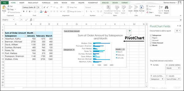
Pivot charts are used to graphically summarize the data and explore complicated data.

A Pivot chart shows the data series, categories, and chart axes the same way a standard chart does. Additionally, it also gives you interactive filtering controls right on the chart so that you can quickly analyze a subset of your data.

Pivot charts are useful when you have the data in a huge Pivot table or a lot of complex worksheet data that includes text and numbers. A Pivot chart can help you make sense of this data.

You can create a Pivot chart in the following ways −

From a Pivot table
From a data table as a standalone without Pivot table
From a data table as a standalone without Pivot table with recommended charts

Creating a PivotChart from a PivotTable

To create a Pivot chart from a Pivot table −

Step 1 − Click the Pivot table. The Ribbon shows the Pivot table tools – ANALYZE and DESIGN on the Ribbon.

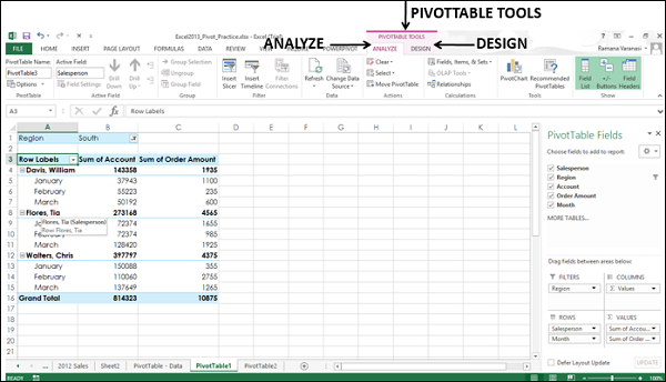
Step 2 − Click the ANALYZE tab. The Ribbon converts to the options available in ANALYZE tab.

Step 3 − Click PivotChart. An Insert Chart window appears.

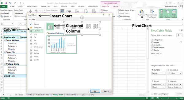
Step 4 − Click Column and then Clustered Column. Click OK. You can see the Pivot chart.

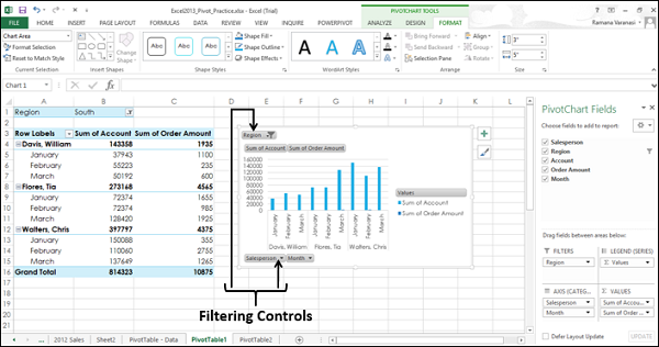
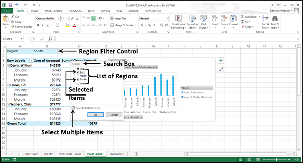
To summarize the data as you want, you can click any interactive control and then pick the sort or filtering options you want.

Step 5 − Click Region Filter Control. A search box appears with the list of all the regions.

Step 6 − Click Select Multiple Items. Check Boxes appear for the list of all the regions.

Step 7 − Select the East and South check boxes. Click OK.

Step 8 − Click the Chart Elements icon.

Step 9 − Click Bottom from the options under the Legend option.

Step 10 − Now click the Month Filter control and select January. Click OK.

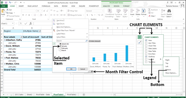
The Pivot chart is displayed with the filtered data.

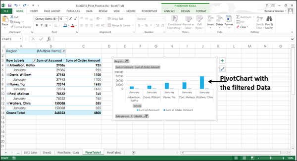
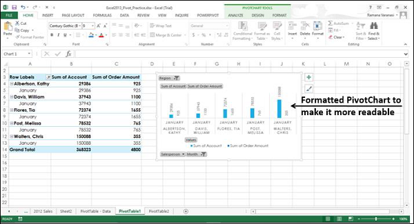
As in the case of normal charts, you can use the chart elements and the chart filters that appear at the right-top corner of the pivot chart to format the pivot chart to make it more presentable.

You have already seen how we changed the position of legend in the above given steps. Now, we will use chart styles to make the Pivot chart much more presentable.

Step 1 − Click the Chart Styles icon.

Step 2 − Under the STYLE option, choose Style 2.

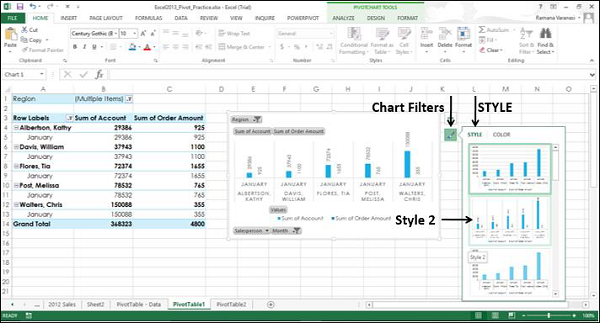
Style 2 has data labels above the columns that makes the Pivot chart more readable.

Creating a PivotChart from the Data Table as a Standalone PivotChart

You can create a Pivot chart without creating a Pivot table first.

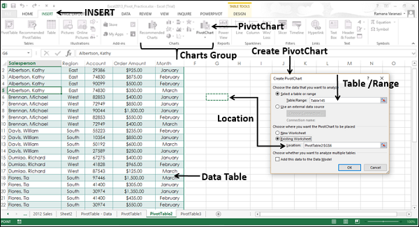
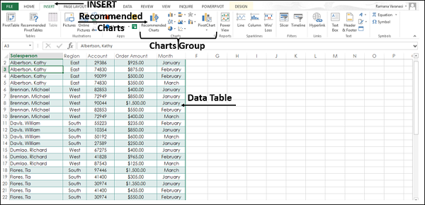
Step 1 − Select the data table.

Step 2 − On the Insert tab, in the Charts group, click PivotChart on the Ribbon.

A Create PivotChart window appears.

Step 3 − Select the Table/Range

Step 4 − Select the location where you want the Pivot chart to be placed. You can choose a cell on the existing worksheet itself or on a new worksheet. Click OK.

An empty Pivot chart and an empty Pivot table appear along with the Pivot chart field list to build the Pivot chart.

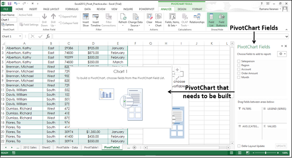
Step 5 − Choose the fields to be added to the Pivot chart.

Step 6 − Arrange the fields by dragging them into FILTERS, LEGEND (SERIES), AXIS (CATEGORIES) and VALUES.

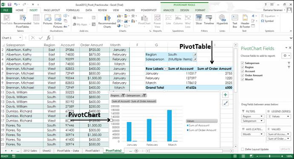
Step 7 − Use the Filter Controls on the Pivot chart to select the data to be placed on the Pivot chart. Excel will automatically create a coupled Pivot table.

Recommended Pivot Charts

You can create a Pivot chart that is recommended for your data without first creating a Pivot table. Just as in the case of normal charts, Excel provides Recommended Pivot charts so that to quickly decide on the type of PivotChart that suits your data.

Step 1 − Select the data table.

Step 2 − On the Insert tab, in the Charts group, click Recommended Charts.

An Insert Chart window appears with two tabs Recommended charts and All charts.

Step 3 − Click the Recommended Charts tab.

Charts with the PivotChart icon in the top right corner are Pivot charts.

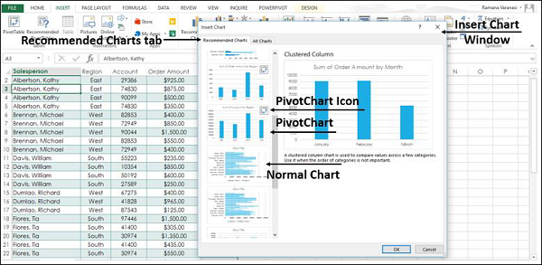
Step 4 − Click a Pivot chart. The preview appears on the right side.

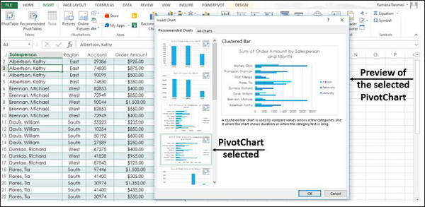
Step 5 − Click OK once you find the Pivot chart you want.

Your standalone Pivot chart for your data is displayed. Excel will automatically create a coupled Pivot table.