Excel Charts - Chart Filters

---

---

You can use Chart Filters to edit the data points (values) and names that are visible on the displayed chart, dynamically.

Step 1 − Click on the chart.

Step 2 − Click the Chart Filters icon that appears at the upper-right corner of the chart. Two tabs – VALUES and NAMES appear in a new window.

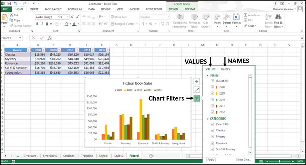
Values

Values are the series and the categories in the data.

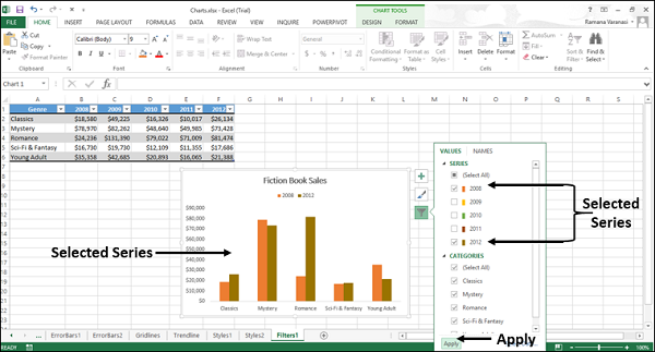
Click the Values tab. The available SERIES and CATEGORIES in your data appear.

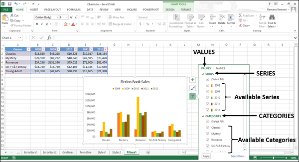
Values – Series

Step 1 − Point on any of the available series. That particular series will be highlighted on the chart. In addition, the data corresponding to that series will be highlighted in the excel table.

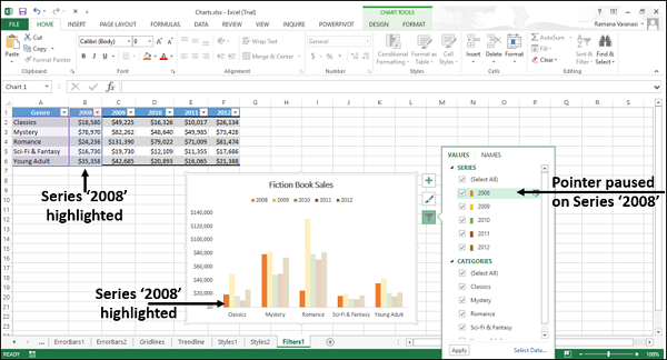
Step 2 − Select the series you want to display and deselect the rest of the series. Click Apply. Only the selected series will be displayed on the chart.

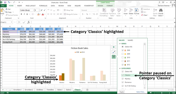
Values – Categories

Step 1 − Point to any of the available categories. That particular category will be highlighted on the chart. In addition, the data corresponding to that category will be highlighted in the excel table.

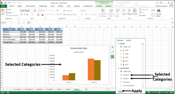
Step 2 − Select the category you want to display deselect the rest of the categories. Click Apply. Only the selected categories will be displayed on the chart.

Names

NAMES represent the names of the series in the chart. By default, names are taken from the excel table.

You can change the names of the series in the chart using the names tab in the chart filters. Click the NAMES tab in the Chart Filters. The names of the series and the names of the categories in the chart will be displayed.

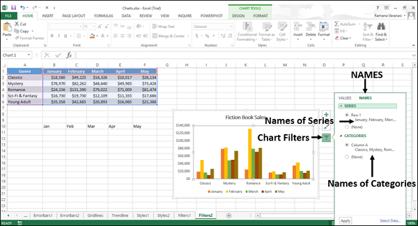
You can change the names of the series and categories with select data button, in the lower right corner of the chart filters box.

Names – Series

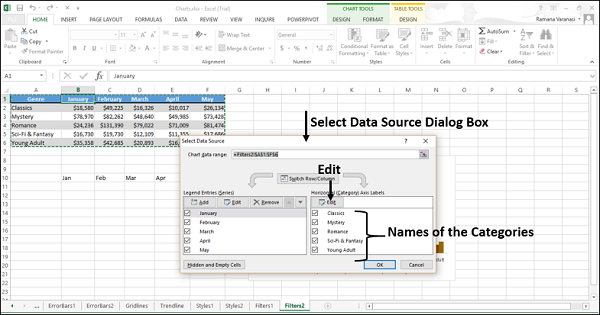
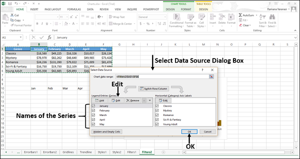
Step 1 − Click the Select Data button. The Select Data Source Dialog Box appears. The names of the series are at the left side of the dialog box.

To change the names of the series,

Step 2 − Click the Edit button above the series names.

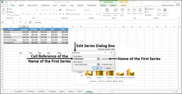
The Edit Series dialog box appears. You can also see the cell reference of the name of the first series.

Step 3 − Change the cell reference of the name of the first series. Click OK.

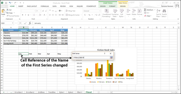
You can see that the name of the first series has changed.

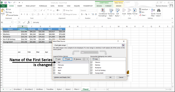
Step 4 − Repeat the steps 2 and 3 for the names of the rest of the series.

Note that the names have changed only in the chart. They have not changed in the Excel table.

Names – Categories

To change the names of the categories, you need to follow the same steps as for series, by selecting the edit button above the categories names in the select data source dialog-box.