- Distributed DBMS Tutorial
- DDBMS - Home
- DDBMS - DBMS Concepts
- DDBMS - Distributed Databases
- Distributed Database Design
- Distributed Database Environments
- DDBMS - Design Strategies
- DDBMS - Distribution Transparency
- DDBMS - Database Control
- Query Optimization
- Relational Algebra Query
- Query Optimization Centralized
- Query Optimization in Distributed
- Concurrency Control
- Transaction Processing Systems
- DDBMS - Controlling Concurrency
- DDBMS - Deadlock Handling
- Failure and Recovery
- DDBMS - Replication Control
- DDBMS - Failure & Commit
- DDBMS - Database Recovery
- Distributed Commit Protocols
- Distributed DBMS Security
- Database Security & Cryptography
- Security in Distributed Databases
- Distributed DBMS Resources
- DDBMS - Quick Guide
- DDBMS - Useful Resources
- DDBMS - Discussion
Relational Algebra for Query Optimization
When a query is placed, it is at first scanned, parsed and validated. An internal representation of the query is then created such as a query tree or a query graph. Then alternative execution strategies are devised for retrieving results from the database tables. The process of choosing the most appropriate execution strategy for query processing is called query optimization.
Query Optimization Issues in DDBMS
In DDBMS, query optimization is a crucial task. The complexity is high since number of alternative strategies may increase exponentially due to the following factors −
- The presence of a number of fragments.
- Distribution of the fragments or tables across various sites.
- The speed of communication links.
- Disparity in local processing capabilities.
Hence, in a distributed system, the target is often to find a good execution strategy for query processing rather than the best one. The time to execute a query is the sum of the following −
- Time to communicate queries to databases.
- Time to execute local query fragments.
- Time to assemble data from different sites.
- Time to display results to the application.
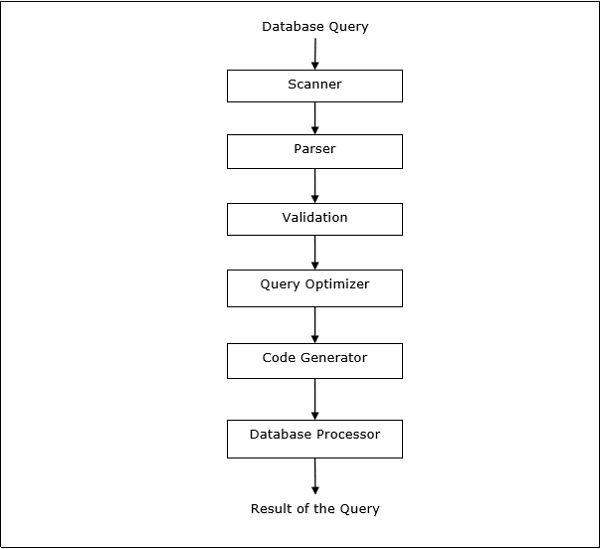
Query Processing
Query processing is a set of all activities starting from query placement to displaying the results of the query. The steps are as shown in the following diagram −
Relational Algebra
Relational algebra defines the basic set of operations of relational database model. A sequence of relational algebra operations forms a relational algebra expression. The result of this expression represents the result of a database query.
The basic operations are −
- Projection
- Selection
- Union
- Intersection
- Minus
- Join
Projection
Projection operation displays a subset of fields of a table. This gives a vertical partition of the table.
Syntax in Relational Algebra
$$\pi_{<{AttributeList}>}{(<{Table Name}>)}$$
For example, let us consider the following Student database −
| Roll_No | Name | Course | Semester | Gender |
| 2 | Amit Prasad | BCA | 1 | Male |
| 4 | Varsha Tiwari | BCA | 1 | Female |
| 5 | Asif Ali | MCA | 2 | Male |
| 6 | Joe Wallace | MCA | 1 | Male |
| 8 | Shivani Iyengar | BCA | 1 | Female |
If we want to display the names and courses of all students, we will use the following relational algebra expression −
$$\pi_{Name,Course}{(STUDENT)}$$
Selection
Selection operation displays a subset of tuples of a table that satisfies certain conditions. This gives a horizontal partition of the table.
Syntax in Relational Algebra
$$\sigma_{<{Conditions}>}{(<{Table Name}>)}$$
For example, in the Student table, if we want to display the details of all students who have opted for MCA course, we will use the following relational algebra expression −
$$\sigma_{Course} = {\small "BCA"}^{(STUDENT)}$$
Combination of Projection and Selection Operations
For most queries, we need a combination of projection and selection operations. There are two ways to write these expressions −
- Using sequence of projection and selection operations.
- Using rename operation to generate intermediate results.
For example, to display names of all female students of the BCA course −
- Relational algebra expression using sequence of projection and selection operations
$$\pi_{Name}(\sigma_{Gender = \small "Female" AND \: Course = \small "BCA"}{(STUDENT)})$$
- Relational algebra expression using rename operation to generate intermediate results
$$FemaleBCAStudent \leftarrow \sigma_{Gender = \small "Female" AND \: Course = \small "BCA"} {(STUDENT)}$$
$$Result \leftarrow \pi_{Name}{(FemaleBCAStudent)}$$
Union
If P is a result of an operation and Q is a result of another operation, the union of P and Q ($p \cup Q$) is the set of all tuples that is either in P or in Q or in both without duplicates.
For example, to display all students who are either in Semester 1 or are in BCA course −
$$Sem1Student \leftarrow \sigma_{Semester = 1}{(STUDENT)}$$
$$BCAStudent \leftarrow \sigma_{Course = \small "BCA"}{(STUDENT)}$$
$$Result \leftarrow Sem1Student \cup BCAStudent$$
Intersection
If P is a result of an operation and Q is a result of another operation, the intersection of P and Q ( $p \cap Q$ ) is the set of all tuples that are in P and Q both.
For example, given the following two schemas −
EMPLOYEE
| EmpID | Name | City | Department | Salary |
PROJECT
| PId | City | Department | Status |
To display the names of all cities where a project is located and also an employee resides −
$$CityEmp \leftarrow \pi_{City}{(EMPLOYEE)}$$
$$CityProject \leftarrow \pi_{City}{(PROJECT)}$$
$$Result \leftarrow CityEmp \cap CityProject$$
Minus
If P is a result of an operation and Q is a result of another operation, P - Q is the set of all tuples that are in P and not in Q.
For example, to list all the departments which do not have an ongoing project (projects with status = ongoing) −
$$AllDept \leftarrow \pi_{Department}{(EMPLOYEE)}$$
$$ProjectDept \leftarrow \pi_{Department} (\sigma_{Status = \small "ongoing"}{(PROJECT)})$$
$$Result \leftarrow AllDept - ProjectDept$$
Join
Join operation combines related tuples of two different tables (results of queries) into a single table.
For example, consider two schemas, Customer and Branch in a Bank database as follows −
CUSTOMER
| CustID | AccNo | TypeOfAc | BranchID | DateOfOpening |
BRANCH
| BranchID | BranchName | IFSCcode | Address |
To list the employee details along with branch details −
$$Result \leftarrow CUSTOMER \bowtie_{Customer.BranchID=Branch.BranchID}{BRANCH}$$
Translating SQL Queries into Relational Algebra
SQL queries are translated into equivalent relational algebra expressions before optimization. A query is at first decomposed into smaller query blocks. These blocks are translated to equivalent relational algebra expressions. Optimization includes optimization of each block and then optimization of the query as a whole.
Examples
Let us consider the following schemas −
EMPLOYEE
| EmpID | Name | City | Department | Salary |
PROJECT
| PId | City | Department | Status |
WORKS
| EmpID | PID | Hours |
Example 1
To display the details of all employees who earn a salary LESS than the average salary, we write the SQL query −
SELECT * FROM EMPLOYEE
WHERE SALARY < ( SELECT AVERAGE(SALARY) FROM EMPLOYEE ) ;
This query contains one nested sub-query. So, this can be broken down into two blocks.
The inner block is −
SELECT AVERAGE(SALARY)FROM EMPLOYEE ;
If the result of this query is AvgSal, then outer block is −
SELECT * FROM EMPLOYEE WHERE SALARY < AvgSal;
Relational algebra expression for inner block −
$$AvgSal \leftarrow \Im_{AVERAGE(Salary)}{EMPLOYEE}$$
Relational algebra expression for outer block −
$$\sigma_{Salary <{AvgSal}>}{EMPLOYEE}$$
Example 2
To display the project ID and status of all projects of employee 'Arun Kumar', we write the SQL query −
SELECT PID, STATUS FROM PROJECT
WHERE PID = ( SELECT FROM WORKS  WHERE EMPID = ( SELECT EMPID FROM EMPLOYEE
            WHERE NAME = 'ARUN KUMAR'));
This query contains two nested sub-queries. Thus, can be broken down into three blocks, as follows −
SELECT EMPID FROM EMPLOYEE WHERE NAME = 'ARUN KUMAR';
SELECT PID FROM WORKS WHERE EMPID = ArunEmpID;
SELECT PID, STATUS FROM PROJECT WHERE PID = ArunPID;
(Here ArunEmpID and ArunPID are the results of inner queries)
Relational algebra expressions for the three blocks are −
$$ArunEmpID \leftarrow \pi_{EmpID}(\sigma_{Name = \small "Arun Kumar"} {(EMPLOYEE)})$$
$$ArunPID \leftarrow \pi_{PID}(\sigma_{EmpID = \small "ArunEmpID"} {(WORKS)})$$
$$Result \leftarrow \pi_{PID, Status}(\sigma_{PID = \small "ArunPID"} {(PROJECT)})$$
Computation of Relational Algebra Operators
The computation of relational algebra operators can be done in many different ways, and each alternative is called an access path.
The computation alternative depends upon three main factors −
- Operator type
- Available memory
- Disk structures
The time to perform execution of a relational algebra operation is the sum of −
- Time to process the tuples.
- Time to fetch the tuples of the table from disk to memory.
Since the time to process a tuple is very much smaller than the time to fetch the tuple from the storage, particularly in a distributed system, disk access is very often considered as the metric for calculating cost of relational expression.
Computation of Selection
Computation of selection operation depends upon the complexity of the selection condition and the availability of indexes on the attributes of the table.
Following are the computation alternatives depending upon the indexes −
No Index − If the table is unsorted and has no indexes, then the selection process involves scanning all the disk blocks of the table. Each block is brought into the memory and each tuple in the block is examined to see whether it satisfies the selection condition. If the condition is satisfied, it is displayed as output. This is the costliest approach since each tuple is brought into memory and each tuple is processed.
B+ Tree Index − Most database systems are built upon the B+ Tree index. If the selection condition is based upon the field, which is the key of this B+ Tree index, then this index is used for retrieving results. However, processing selection statements with complex conditions may involve a larger number of disk block accesses and in some cases complete scanning of the table.
Hash Index − If hash indexes are used and its key field is used in the selection condition, then retrieving tuples using the hash index becomes a simple process. A hash index uses a hash function to find the address of a bucket where the key value corresponding to the hash value is stored. In order to find a key value in the index, the hash function is executed and the bucket address is found. The key values in the bucket are searched. If a match is found, the actual tuple is fetched from the disk block into the memory.
Computation of Joins
When we want to join two tables, say P and Q, each tuple in P has to be compared with each tuple in Q to test if the join condition is satisfied. If the condition is satisfied, the corresponding tuples are concatenated, eliminating duplicate fields and appended to the result relation. Consequently, this is the most expensive operation.
The common approaches for computing joins are −
Nested-loop Approach
This is the conventional join approach. It can be illustrated through the following pseudocode (Tables P and Q, with tuples tuple_p and tuple_q and joining attribute a) −
For each tuple_p in P
For each tuple_q in Q
If tuple_p.a = tuple_q.a Then
   Concatenate tuple_p and tuple_q and append to Result
End If
Next tuple_q
Next tuple-p
Sort-merge Approach
In this approach, the two tables are individually sorted based upon the joining attribute and then the sorted tables are merged. External sorting techniques are adopted since the number of records is very high and cannot be accommodated in the memory. Once the individual tables are sorted, one page each of the sorted tables are brought to the memory, merged based upon the joining attribute and the joined tuples are written out.
Hash-join Approach
This approach comprises of two phases: partitioning phase and probing phase. In partitioning phase, the tables P and Q are broken into two sets of disjoint partitions. A common hash function is decided upon. This hash function is used to assign tuples to partitions. In the probing phase, tuples in a partition of P are compared with the tuples of corresponding partition of Q. If they match, then they are written out.