- Digital Signal Processing Tutorial
- DSP - Home
- DSP - Signals-Definition
- DSP - Basic CT Signals
- DSP - Basic DT Signals
- DSP - Classification of CT Signals
- DSP - Classification of DT Signals
- DSP - Miscellaneous Signals
- Operations on Signals
- Operations Signals - Shifting
- Operations Signals - Scaling
- Operations Signals - Reversal
- Operations Signals - Differentiation
- Operations Signals - Integration
- Operations Signals - Convolution
- Basic System Properties
- DSP - Static Systems
- DSP - Dynamic Systems
- DSP - Causal Systems
- DSP - Non-Causal Systems
- DSP - Anti-Causal Systems
- DSP - Linear Systems
- DSP - Non-Linear Systems
- DSP - Time-Invariant Systems
- DSP - Time-Variant Systems
- DSP - Stable Systems
- DSP - Unstable Systems
- DSP - Solved Examples
- Z-Transform
- Z-Transform - Introduction
- Z-Transform - Properties
- Z-Transform - Existence
- Z-Transform - Inverse
- Z-Transform - Solved Examples
- Discrete Fourier Transform
- DFT - Introduction
- DFT - Time Frequency Transform
- DTF - Circular Convolution
- DFT - Linear Filtering
- DFT - Sectional Convolution
- DFT - Discrete Cosine Transform
- DFT - Solved Examples
- Fast Fourier Transform
- DSP - Fast Fourier Transform
- DSP - In-Place Computation
- DSP - Computer Aided Design
- Digital Signal Processing Resources
- DSP - Quick Guide
- DSP - Useful Resources
- DSP - Discussion
DSP - Computer Aided Design
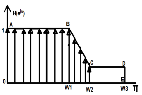
FIR filters can be useful in making computer-aided design of the filters. Let us take an example and see how it works. Given below is a figure of desired filter.
While doing computer designing, we break the whole continuous graph figures into discrete values. Within certain limits, we break it into either 64, 256 or 512 (and so on) number of parts having discrete magnitudes.
In the above example, we have taken limits between -π to +π. We have divided it into 256 parts. The points can be represented as H(0), H(1),….up to H(256). Here, we apply IDFT algorithm and this will give us linear phase characteristics.
Sometimes, we may be interested in some particular order of filter. Let us say we want to realize the above given design through 9th order filter. So, we take filter values as h0, h1, h2….h9. Mathematically, it can be shown as below
$$H(e^{j\omega}) = h_0+h_1e^{-j\omega}+h_2e^{-2j\omega}+.....+h_9e^{-9j\omega}$$Where there are large number of dislocations, we take maximum points.
For example, in the above figure, there is a sudden drop of slopping between the points B and C. So, we try to take more discrete values at this point, but there is a constant slope between point C and D. There we take less number of discrete values.
For designing the above filter, we go through minimization process as follows;
$H(e^{j\omega1}) = h_0+h_1e^{-j\omega1}+h_2e^{-2j\omega1}+.....+h_9e^{-9j\omega1}$
$H(e^{j\omega2}) = h_0+h_1e^{-j\omega2}+h_2e^{-2j\omega2}+.....+h_9e^{-9j\omega2}$
Similarly,
$(e^{j\omega1000}) = h_0+h_1eH^{-j\omega1000}h_2e^{-2j\omega1000}+.....+h_9+e^{-9j\omega1000}$
Representing the above equation in matrix form, we have −
$$\begin{bmatrix}H(e^{j\omega_1})\\.\\.\\H(e^{j\omega_{1000}}) \end{bmatrix} = \begin{bmatrix}e^{-j\omega_1} & ... & e^{-j9\omega_1} \\. & & . \\. & & . \\e^{-j\omega_{1000}} &... & e^{j9\omega_{1000}} \end{bmatrix}\begin{bmatrix}h_0\\.\\.\\h_9\end{bmatrix}$$Let us take the 1000×1 matrix as B, 1000×9 matrix as A and 9×1 matrix as $\hat{h}$.
So, for solving the above matrix, we will write
$\hat{h} = [A^TA]^{-1}A^{T}B$
$= [A^{*T}A]^{-1}A^{*T}B$
where A* represents the complex conjugate of the matrix A.