- Digital Signal Processing Tutorial
- DSP - Home
- DSP - Signals-Definition
- DSP - Basic CT Signals
- DSP - Basic DT Signals
- DSP - Classification of CT Signals
- DSP - Classification of DT Signals
- DSP - Miscellaneous Signals
- Operations on Signals
- Operations Signals - Shifting
- Operations Signals - Scaling
- Operations Signals - Reversal
- Operations Signals - Differentiation
- Operations Signals - Integration
- Operations Signals - Convolution
- Basic System Properties
- DSP - Static Systems
- DSP - Dynamic Systems
- DSP - Causal Systems
- DSP - Non-Causal Systems
- DSP - Anti-Causal Systems
- DSP - Linear Systems
- DSP - Non-Linear Systems
- DSP - Time-Invariant Systems
- DSP - Time-Variant Systems
- DSP - Stable Systems
- DSP - Unstable Systems
- DSP - Solved Examples
- Z-Transform
- Z-Transform - Introduction
- Z-Transform - Properties
- Z-Transform - Existence
- Z-Transform - Inverse
- Z-Transform - Solved Examples
- Discrete Fourier Transform
- DFT - Introduction
- DFT - Time Frequency Transform
- DTF - Circular Convolution
- DFT - Linear Filtering
- DFT - Sectional Convolution
- DFT - Discrete Cosine Transform
- DFT - Solved Examples
- Fast Fourier Transform
- DSP - Fast Fourier Transform
- DSP - In-Place Computation
- DSP - Computer Aided Design
- Digital Signal Processing Resources
- DSP - Quick Guide
- DSP - Useful Resources
- DSP - Discussion
Digital Signal Processing - Quick Guide
Digital Signal Processing - Signals-Definition
Definition
Anything that carries information can be called as signal. It can also be defined as a physical quantity that varies with time, temperature, pressure or with any independent variables such as speech signal or video signal.
The process of operation in which the characteristics of a signal (Amplitude, shape, phase, frequency, etc.) undergoes a change is known as signal processing.
Note − Any unwanted signal interfering with the main signal is termed as noise. So, noise is also a signal but unwanted.
According to their representation and processing, signals can be classified into various categories details of which are discussed below.
Continuous Time Signals
Continuous-time signals are defined along a continuum of time and are thus, represented by a continuous independent variable. Continuous-time signals are often referred to as analog signals.
This type of signal shows continuity both in amplitude and time. These will have values at each instant of time. Sine and cosine functions are the best example of Continuous time signal.
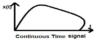
The signal shown above is an example of continuous time signal because we can get value of signal at each instant of time.
Discrete Time signals
The signals, which are defined at discrete times are known as discrete signals. Therefore, every independent variable has distinct value. Thus, they are represented as sequence of numbers.
Although speech and video signals have the privilege to be represented in both continuous and discrete time format; under certain circumstances, they are identical. Amplitudes also show discrete characteristics. Perfect example of this is a digital signal; whose amplitude and time both are discrete.
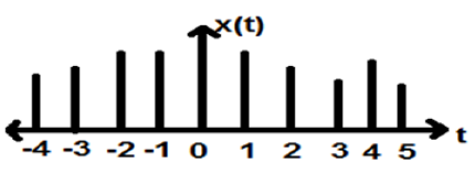
The figure above depicts a discrete signal’s discrete amplitude characteristic over a period of time. Mathematically, these types of signals can be formularized as;
$$x = \left \{ x\left [ n \right ] \right \},\quad -\infty < n< \infty$$Where, n is an integer.
It is a sequence of numbers x, where nth number in the sequence is represented as x[n].
Digital Signal Processing - Basic CT Signals
To test a system, generally, standard or basic signals are used. These signals are the basic building blocks for many complex signals. Hence, they play a very important role in the study of signals and systems.
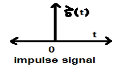
Unit Impulse or Delta Function
A signal, which satisfies the condition, $\delta(t) = \lim_{\epsilon \to \infty} x(t)$ is known as unit impulse signal. This signal tends to infinity when t = 0 and tends to zero when t ≠ 0 such that the area under its curve is always equals to one. The delta function has zero amplitude everywhere excunit_impulse.jpgept at t = 0.
Properties of Unit Impulse Signal
- δ(t) is an even signal.
- δ(t) is an example of neither energy nor power (NENP) signal.
- Area of unit impulse signal can be written as; $$A = \int_{-\infty}^{\infty} \delta (t)dt = \int_{-\infty}^{\infty} \lim_{\epsilon \to 0} x(t) dt = \lim_{\epsilon \to 0} \int_{-\infty}^{\infty} [x(t)dt] = 1$$
- Weight or strength of the signal can be written as; $$y(t) = A\delta (t)$$
- Area of the weighted impulse signal can be written as − $$y (t) = \int_{-\infty}^{\infty} y (t)dt = \int_{-\infty}^{\infty} A\delta (t) = A[\int_{-\infty}^{\infty} \delta (t)dt ] = A = 1 = Wigthedimpulse$$
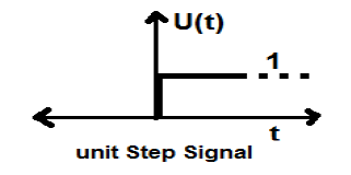
Unit Step Signal
A signal, which satisfies the following two conditions −
- $U(t) = 1(when\quad t \geq 0 )and$
- $U(t) = 0 (when\quad t < 0 )$
is known as a unit step signal.
It has the property of showing discontinuity at t = 0. At the point of discontinuity, the signal value is given by the average of signal value. This signal has been taken just before and after the point of discontinuity (according to Gibb’s Phenomena).
If we add a step signal to another step signal that is time scaled, then the result will be unity. It is a power type signal and the value of power is 0.5. The RMS (Root mean square) value is 0.707 and its average value is also 0.5
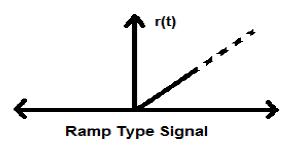
Ramp Signal
Integration of step signal results in a Ramp signal. It is represented by r(t). Ramp signal also satisfies the condition $r(t) = \int_{-\infty}^{t} U(t)dt = tU(t)$. It is neither energy nor power (NENP) type signal.
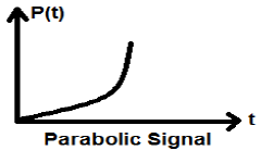
Parabolic Signal
Integration of Ramp signal leads to parabolic signal. It is represented by p(t). Parabolic signal also satisfies he condition $p(t) = \int_{-\infty}^{t} r(t)dt = (t^{2}/2)U(t)$ . It is neither energy nor Power (NENP) type signal.
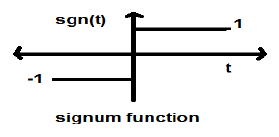
Signum Function
This function is represented as
$$sgn(t) = \begin{cases}1 & for\quad t >0\\-1 & for\quad t<0\end{cases}$$It is a power type signal. Its power value and RMS (Root mean square) values, both are 1. Average value of signum function is zero.
Sinc Function
It is also a function of sine and is written as −
$$SinC(t) = \frac{Sin\Pi t}{\Pi T} = Sa(\Pi t)$$Properties of Sinc function
It is an energy type signal.
$Sinc(0) = \lim_{t \to 0}\frac{\sin \Pi t}{\Pi t} = 1$
$Sinc(\infty) = \lim_{t \to \infty}\frac{\sin \Pi \infty}{\Pi \infty} = 0$ (Range of sinπ∞ varies between -1 to +1 but anything divided by infinity is equal to zero)
-
If $ \sin c(t) = 0 => \sin \Pi t = 0$
$\Rightarrow \Pi t = n\Pi$
$\Rightarrow t = n (n \neq 0)$
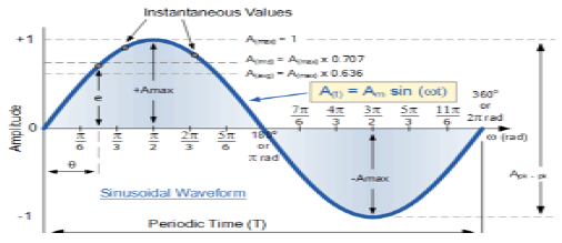
Sinusoidal Signal
A signal, which is continuous in nature is known as continuous signal. General format of a sinusoidal signal is
$$x(t) = A\sin (\omega t + \phi )$$Here,
A = amplitude of the signal
ω = Angular frequency of the signal (Measured in radians)
φ = Phase angle of the signal (Measured in radians)
The tendency of this signal is to repeat itself after certain period of time, thus is called periodic signal. The time period of signal is given as;
$$T = \frac{2\pi }{\omega }$$The diagrammatic view of sinusoidal signal is shown below.
Rectangular Function
A signal is said to be rectangular function type if it satisfies the following condition −
$$\pi(\frac{t}{\tau}) = \begin{cases}1, & for\quad t\leq \frac{\tau}{2}\\0, & Otherwise\end{cases}$$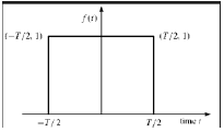
Being symmetrical about Y-axis, this signal is termed as even signal.
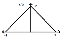
Triangular Pulse Signal
Any signal, which satisfies the following condition, is known as triangular signal.
$$\Delta(\frac{t}{\tau}) = \begin{cases}1-(\frac{2|t|}{\tau}) & for|t|<\frac{\tau}{2}\\0 & for|t|>\frac{\tau}{2}\end{cases}$$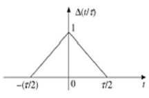
This signal is symmetrical about Y-axis. Hence, it is also termed as even signal.
Digital Signal Processing - Basic DT Signals
We have seen that how the basic signals can be represented in Continuous time domain. Let us see how the basic signals can be represented in Discrete Time Domain.
Unit Impulse Sequence
It is denoted as δ(n) in discrete time domain and can be defined as;
$$\delta(n)=\begin{cases}1, & for \quad n=0\\0, & Otherwise\end{cases}$$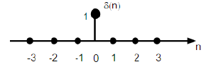
Unit Step Signal
Discrete time unit step signal is defined as;
$$U(n)=\begin{cases}1, & for \quad n\geq0\\0, & for \quad n<0\end{cases}$$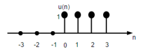
The figure above shows the graphical representation of a discrete step function.
Unit Ramp Function
A discrete unit ramp function can be defined as −
$$r(n)=\begin{cases}n, & for \quad n\geq0\\0, & for \quad n<0\end{cases}$$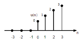
The figure given above shows the graphical representation of a discrete ramp signal.
Parabolic Function
Discrete unit parabolic function is denoted as p(n) and can be defined as;
$$p(n) = \begin{cases}\frac{n^{2}}{2} ,& for \quad n\geq0\\0, & for \quad n<0\end{cases}$$In terms of unit step function it can be written as;
$$P(n) = \frac{n^{2}}{2}U(n)$$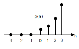
The figure given above shows the graphical representation of a parabolic sequence.
Sinusoidal Signal
All continuous-time signals are periodic. The discrete-time sinusoidal sequences may or may not be periodic. They depend on the value of ω. For a discrete time signal to be periodic, the angular frequency ω must be a rational multiple of 2π.
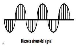
A discrete sinusoidal signal is shown in the figure above.
Discrete form of a sinusoidal signal can be represented in the format −
$$x(n) = A\sin(\omega n + \phi)$$Here A,ω and φ have their usual meaning and n is the integer. Time period of the discrete sinusoidal signal is given by −
$$N =\frac{2\pi m}{\omega}$$Where, N and m are integers.
DSP - Classification of CT Signals
Continuous time signals can be classified according to different conditions or operations performed on the signals.
Even and Odd Signals
Even Signal
A signal is said to be even if it satisfies the following condition;
$$x(-t) = x(t)$$Time reversal of the signal does not imply any change on amplitude here. For example, consider the triangular wave shown below.
The triangular signal is an even signal. Since, it is symmetrical about Y-axis. We can say it is mirror image about Y-axis.
Consider another signal as shown in the figure below.
We can see that the above signal is even as it is symmetrical about Y-axis.
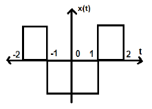
Odd Signal
A signal is said to be odd, if it satisfies the following condition
$$x(-t) = -x(t)$$Here, both the time reversal and amplitude change takes place simultaneously.
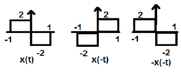
In the figure above, we can see a step signal x(t). To test whether it is an odd signal or not, first we do the time reversal i.e. x(-t) and the result is as shown in the figure. Then we reverse the amplitude of the resultant signal i.e. –x(-t) and we get the result as shown in figure.
If we compare the first and the third waveform, we can see that they are same, i.e. x(t)= -x(-t), which satisfies our criteria. Therefore, the above signal is an Odd signal.
Some important results related to even and odd signals are given below.
- Even × Even = Even
- Odd × Odd = Even
- Even × Odd = Odd
- Even ± Even = Even
- Odd ± Odd = Odd
- Even ± Odd = Neither even nor odd
Representation of any signal into even or odd form
Some signals cannot be directly classified into even or odd type. These are represented as a combination of both even and odd signal.
$$x(t)\rightarrow x_{e}(t)+x_{0}(t)$$Where xe(t) represents the even signal and xo(t) represents the odd signal
$$x_{e}(t)=\frac{[x(t)+x(-t)]}{2}$$And
$$x_{0}(t)=\frac{[x(t)-x(-t)]}{2}$$Example
Find the even and odd parts of the signal $x(n) = t+t^{2}+t^{3}$
Solution − From reversing x(n), we get
$$x(-n) = -t+t^{2}-t^{3}$$
Now, according to formula, the even part
$$x_{e}(t) = \frac{x(t)+x(-t)}{2}$$
$$= \frac{[(t+t^{2}+t^{3})+(-t+t^{2}-t^{3})]}{2}$$
$$= t^{2}$$
Similarly, according to formula the odd part is
$$x_{0}(t)=\frac{[x(t)-x(-t)]}{2}$$
$$= \frac{[(t+t^{2}+t^{3})-(-t+t^{2}-t^{3})]}{2}$$
$$= t+t^{3}$$
Periodic and Non-Periodic Signals
Periodic Signals
Periodic signal repeats itself after certain interval of time. We can show this in equation form as −
$$x(t) = x(t)\pm nT$$Where, n = an integer (1,2,3……)
T = Fundamental time period (FTP) ≠ 0 and ≠∞
Fundamental time period (FTP) is the smallest positive and fixed value of time for which signal is periodic.
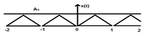
A triangular signal is shown in the figure above of amplitude A. Here, the signal is repeating after every 1 sec. Therefore, we can say that the signal is periodic and its FTP is 1 sec.
Non-Periodic Signal
Simply, we can say, the signals, which are not periodic are non-periodic in nature. As obvious, these signals will not repeat themselves after any interval time.
Non-periodic signals do not follow a certain format; therefore, no particular mathematical equation can describe them.
Energy and Power Signals
A signal is said to be an Energy signal, if and only if, the total energy contained is finite and nonzero (0<E<∞). Therefore, for any energy type signal, the total normalized signal is finite and non-zero.
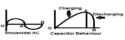
A sinusoidal AC current signal is a perfect example of Energy type signal because it is in positive half cycle in one case and then is negative in the next half cycle. Therefore, its average power becomes zero.
A lossless capacitor is also a perfect example of Energy type signal because when it is connected to a source it charges up to its optimum level and when the source is removed, it dissipates that equal amount of energy through a load and makes its average power to zero.
For any finite signal x(t) the energy can be symbolized as E and is written as;
$$E = \int_{-\infty}^{+\infty} x^{2}(t)dt$$Spectral density of energy type signals gives the amount of energy distributed at various frequency levels.
Power type Signals
A signal is said to be power type signal, if and only if, normalized average power is finite and non-zero i.e. (0<p<∞). For power type signal, normalized average power is finite and non-zero. Almost all the periodic signals are power signals and their average power is finite and non-zero.
In mathematical form, the power of a signal x(t) can be written as;
$$P = \lim_{T \rightarrow \infty}1/T\int_{-T/2}^{+T/2} x^{2}(t)dt$$Difference between Energy and Power Signals
The following table summarizes the differences of Energy and Power Signals.
| Power signal | Energy Signal |
|---|---|
| Practical periodic signals are power signals. | Non-periodic signals are energy signals. |
| Here, Normalized average power is finite and non-zero. | Here, total normalized energy is finite and non-zero. |
|
Mathematically, $$P = \lim_{T \rightarrow \infty}1/T\int_{-T/2}^{+T/2} x^{2}(t)dt$$ |
Mathematically, $$E = \int_{-\infty}^{+\infty} x^{2}(t)dt$$ |
| Existence of these signals is infinite over time. | These signals exist for limited period of time. |
| Energy of power signal is infinite over infinite time. | Power of the energy signal is zero over infinite time. |
Solved Examples
Example 1 − Find the Power of a signal $z(t) = 2\cos(3\Pi t+30^{o})+4\sin(3\Pi +30^{o})$
Solution − The above two signals are orthogonal to each other because their frequency terms are identical to each other also they have same phase difference. So, total power will be the summation of individual powers.
Let $z(t) = x(t)+y(t)$
Where $x(t) = 2\cos (3\Pi t+30^{o})$ and $y(t) = 4\sin(3\Pi +30^{o})$
Power of $x(t) = \frac{2^{2}}{2} = 2$
Power of $y(t) = \frac{4^{2}}{2} = 8$
Therefore, $P(z) = p(x)+p(y) = 2+8 = 10$…Ans.
Example 2 − Test whether the signal given $x(t) = t^{2}+j\sin t$ is conjugate or not?
Solution − Here, the real part being t2 is even and odd part (imaginary) being $\sin t$ is odd. So the above signal is Conjugate signal.
Example 3 − Verify whether $X(t)= \sin \omega t$ is an odd signal or an even signal.
Solution − Given $X(t) = \sin \omega t$
By time reversal, we will get $\sin (-\omega t)$
But we know that $\sin(-\phi) = -\sin \phi$.
Therefore,
$$\sin (-\omega t) = -\sin \omega t$$This is satisfying the condition for a signal to be odd. Therefore, $\sin \omega t$ is an odd signal.
DSP - Classification of DT Signals
Just like Continuous time signals, Discrete time signals can be classified according to the conditions or operations on the signals.
Even and Odd Signals
Even Signal
A signal is said to be even or symmetric if it satisfies the following condition;
$$x(-n) = x(n)$$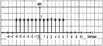
Here, we can see that x(-1) = x(1), x(-2) = x(2) and x(-n) = x(n). Thus, it is an even signal.
Odd Signal
A signal is said to be odd if it satisfies the following condition;
$$x(-n) = -x(n)$$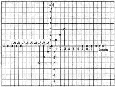
From the figure, we can see that x(1) = -x(-1), x(2) = -x(2) and x(n) = -x(-n). Hence, it is an odd as well as anti-symmetric signal.
Periodic and Non-Periodic Signals
A discrete time signal is periodic if and only if, it satisfies the following condition −
$$x(n+N) = x(n)$$Here, x(n) signal repeats itself after N period. This can be best understood by considering a cosine signal −
$$x(n) = A \cos(2\pi f_{0}n+\theta)$$ $$x(n+N) = A\cos(2\pi f_{0}(n+N)+\theta) = A\cos(2\pi f_{0}n+2\pi f_{0}N+\theta)$$ $$= A\cos(2\pi f_{0}n+2\pi f_{0}N+\theta)$$For the signal to become periodic, following condition should be satisfied;
$$x(n+N) = x(n)$$ $$\Rightarrow A\cos(2\pi f_{0}n+2\pi f_{0}N+\theta) = A \cos(2\pi f_{0}n+\theta)$$i.e. $2\pi f_{0}N$ is an integral multiple of $2\pi$
$$2\pi f_{0}N = 2\pi K$$ $$\Rightarrow N = \frac{K}{f_{0}}$$Frequencies of discrete sinusoidal signals are separated by integral multiple of $2\pi$.
Energy and Power Signals
Energy Signal
Energy of a discrete time signal is denoted as E. Mathematically, it can be written as;
$$E = \displaystyle \sum\limits_{n=-\infty}^{+\infty}|x(n)|^2$$If each individual values of $x(n)$ are squared and added, we get the energy signal. Here $x(n)$ is the energy signal and its energy is finite over time i.e $0< E< \infty$
Power Signal
Average power of a discrete signal is represented as P. Mathematically, this can be written as;
$$P = \lim_{N \to \infty} \frac{1}{2N+1}\displaystyle\sum\limits_{n=-N}^{+N} |x(n)|^2$$Here, power is finite i.e. 0<P<∞. However, there are some signals, which belong to neither energy nor power type signal.
DSP - Miscellaneous Signals
There are other signals, which are a result of operation performed on them. Some common type of signals are discussed below.
Conjugate Signals
Signals, which satisfies the condition $x(t) = x*(-t)$ are called conjugate signals.
Let $x(t) = a(t)+jb(t)$...eqn. 1
So, $x(-t) = a(-t)+jb(-t)$
And $x*(-t) = a(-t)-jb(-t)$...eqn. 2
By Condition, $x(t) = x*(-t)$
If we compare both the derived equations 1 and 2, we can see that the real part is even, whereas the imaginary part is odd. This is the condition for a signal to be a conjugate type.
Conjugate Anti-Symmetric Signals
Signals, which satisfy the condition $x(t) = -x*(-t)$ are called conjugate anti-symmetric signal
Let $x(t) = a(t)+jb(t)$...eqn. 1
So $x(-t) = a(-t)+jb(-t)$
And $x*(-t) = a(-t)-jb(-t)$
$-x*(-t) = -a(-t)+jb(-t)$...eqn. 2
By Condition $x(t) = -x*(-t)$
Now, again compare, both the equations just as we did for conjugate signals. Here, we will find that the real part is odd and the imaginary part is even. This is the condition for a signal to become conjugate anti-symmetric type.
Example
Let the signal given be $x(t) = \sin t+jt^{2}$.
Here, the real part being $\sin t$ is odd and the imaginary part being $t^2$ is even. So, this signal can be classified as conjugate anti-symmetric signal.
Any function can be divided into two parts. One part being Conjugate symmetry and other part being conjugate anti-symmetric. So any signal x(t) can be written as
$$x(t) = xcs(t)+xcas(t)$$Where $xcs(t)$ is conjugate symmetric signal and $xcas(t)$ is conjugate anti symmetric signal
$$xcs(t) = \frac{[x(t)+x*(-t)]}{2}$$And
$$xcas(t) = \frac{[x(t)-x*(-t)]}{2}$$Half Wave Symmetric Signals
When a signal satisfies the condition $cx(t) = -x(t\pm (\frac{T_{0}}{2}))$, it is called half wave symmetric signal. Here, amplitude reversal and time shifting of the signal takes place by half time. For half wave symmetric signal, average value will be zero but this is not the case when the situation is reversed.
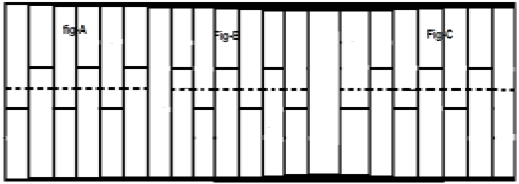
Consider a signal x(t) as shown in figure A above. The first step is to time shift the signal and make it $x[t-(\frac{T}{2})]$. So, the new signal is changed as shown in figure B. Next, we reverse the amplitude of the signal, i.e. make it $-x[t-(\frac{T}{2})]$ as shown in figure C. Since, this signal repeats itself after half-time shifting and reversal of amplitude, it is a half wave symmetric signal.
Orthogonal Signal
Two signals x(t) and y(t) are said to be orthogonal if they satisfy the following two conditions.
Condition 1 − $\int_{-\infty}^{\infty}x(t)y(t) = 0$ [for non-periodic signal]
Condition 2 − $\int x(t)y(t) = 0$ [For periodic Signal]
The signals, which contain odd harmonics (3rd, 5th, 7th ...etc.) and have different frequencies, are mutually orthogonal to each other.
In trigonometric type signals, sine functions and cosine functions are also orthogonal to each other; provided, they have same frequency and are in same phase. In the same manner DC (Direct current signals) and sinusoidal signals are also orthogonal to each other. If x(t) and y(t) are two orthogonal signals and $z(t) = x(t)+y(t)$ then the power and energy of z(t) can be written as ;
$$P(z) = p(x)+p(y)$$ $$E(z) = E(x)+E(y)$$Example
Analyze the signal: $z(t) = 3+4\sin(2\pi t+30^0)$
Here, the signal comprises of a DC signal (3) and one sine function. So, by property this signal is an orthogonal signal and the two sub-signals in it are mutually orthogonal to each other.
DSP - Operations on Signals Shifting
Shifting means movement of the signal, either in time domain (around Y-axis) or in amplitude domain (around X-axis). Accordingly, we can classify the shifting into two categories named as Time shifting and Amplitude shifting, these are subsequently discussed below.
Time Shifting
Time shifting means, shifting of signals in the time domain. Mathematically, it can be written as
$$x(t) \rightarrow y(t+k)$$This K value may be positive or it may be negative. According to the sign of k value, we have two types of shifting named as Right shifting and Left shifting.
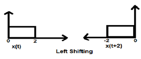
Case 1 (K > 0)
When K is greater than zero, the shifting of the signal takes place towards "left" in the time domain. Therefore, this type of shifting is known as Left Shifting of the signal.
Example
Case 2 (K < 0)
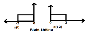
When K is less than zero the shifting of signal takes place towards right in the time domain. Therefore, this type of shifting is known as Right shifting.
Example
The figure given below shows right shifting of a signal by 2.
Amplitude Shifting
Amplitude shifting means shifting of signal in the amplitude domain (around X-axis). Mathematically, it can be represented as −
$$x(t) \rightarrow x(t)+K$$This K value may be positive or negative. Accordingly, we have two types of amplitude shifting which are subsequently discussed below.
Case 1 (K > 0)
When K is greater than zero, the shifting of signal takes place towards up in the x-axis. Therefore, this type of shifting is known as upward shifting.
Example
Let us consider a signal x(t) which is given as;
$$x = \begin{cases}0, & t < 0\\1, & 0\leq t\leq 2\\ 0, & t>0\end{cases}$$Let we have taken K=+1 so new signal can be written as −
$y(t) \rightarrow x(t)+1$ So, y(t) can finally be written as;
$$x(t) = \begin{cases}1, & t < 0\\2, & 0\leq t\leq 2\\ 1, & t>0\end{cases}$$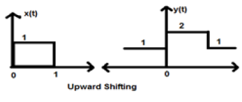
Case 2 (K < 0)
When K is less than zero shifting of signal takes place towards downward in the X- axis. Therefore, it is called downward shifting of the signal.
Example
Let us consider a signal x(t) which is given as;
$$x(t) = \begin{cases}0, & t < 0\\1, & 0\leq t\leq 2\\ 0, & t>0\end{cases}$$Let we have taken K = -1 so new signal can be written as;
$y(t)\rightarrow x(t)-1$ So, y(t) can finally be written as;
$$y(t) = \begin{cases}-1, & t < 0\\0, & 0\leq t\leq 2\\ -1, & t>0\end{cases}$$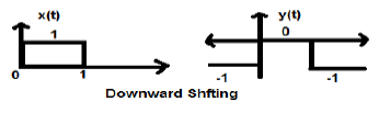
DSP - Operations on Signals Scaling
Scaling of a signal means, a constant is multiplied with the time or amplitude of the signal.
Time Scaling
If a constant is multiplied to the time axis then it is known as Time scaling. This can be mathematically represented as;
$x(t) \rightarrow y(t) = x(\alpha t)$ or $x(\frac{t}{\alpha})$; where α ≠ 0
So the y-axis being same, the x- axis magnitude decreases or increases according to the sign of the constant (whether positive or negative). Therefore, scaling can also be divided into two categories as discussed below.
Time Compression
Whenever alpha is greater than zero, the signal’s amplitude gets divided by alpha whereas the value of the Y-axis remains the same. This is known as Time Compression.
Example
Let us consider a signal x(t), which is shown as in figure below. Let us take the value of alpha as 2. So, y(t) will be x(2t), which is illustrated in the given figure.
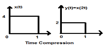
Clearly, we can see from the above figures that the time magnitude in y-axis remains the same but the amplitude in x-axis reduces from 4 to 2. Therefore, it is a case of Time Compression.
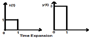
Time Expansion
When the time is divided by the constant alpha, the Y-axis magnitude of the signal get multiplied alpha times, keeping X-axis magnitude as it is. Therefore, this is called Time expansion type signal.
Example
Let us consider a square signal x(t), of magnitude 1. When we time scaled it by a constant 3, such that $x(t) \rightarrow y(t) \rightarrow x(\frac{t}{3})$, then the signal’s amplitude gets modified by 3 times which is shown in the figure below.
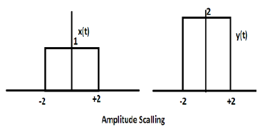
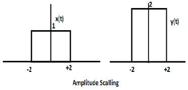
Amplitude Scaling
Multiplication of a constant with the amplitude of the signal causes amplitude scaling. Depending upon the sign of the constant, it may be either amplitude scaling or attenuation. Let us consider a square wave signal x(t) = Π(t/4).
Suppose we define another function y(t) = 2 Π(t/4). In this case, value of y-axis will be doubled, keeping the time axis value as it is. The is illustrated in the figure given below.
Consider another square wave function defined as z(t) where z(t) = 0.5 Π(t/4). Here, amplitude of the function z(t) will be half of that of x(t) i.e. time axis remaining same, amplitude axis will be halved. This is illustrated by the figure given below.
DSP - Operations on Signals Reversal
Whenever the time in a signal gets multiplied by -1, the signal gets reversed. It produces its mirror image about Y or X-axis. This is known as Reversal of the signal.
Reversal can be classified into two types based on the condition whether the time or the amplitude of the signal is multiplied by -1.
Time Reversal
Whenever signal’s time is multiplied by -1, it is known as time reversal of the signal. In this case, the signal produces its mirror image about Y-axis. Mathematically, this can be written as;
$$x(t) \rightarrow y(t) \rightarrow x(-t)$$This can be best understood by the following example.
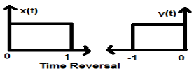
In the above example, we can clearly see that the signal has been reversed about its Y-axis. So, it is one kind of time scaling also, but here the scaling quantity is (-1) always.
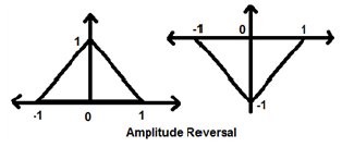
Amplitude Reversal
Whenever the amplitude of a signal is multiplied by -1, then it is known as amplitude reversal. In this case, the signal produces its mirror image about X-axis. Mathematically, this can be written as;
$$x(t)\rightarrow y(t)\rightarrow -x(t)$$Consider the following example. Amplitude reversal can be seen clearly.
DSP - Operations on Signals Differentiation
Two very important operations performed on the signals are Differentiation and Integration.
Differentiation
Differentiation of any signal x(t) means slope representation of that signal with respect to time. Mathematically, it is represented as;
$$x(t)\rightarrow \frac{dx(t)}{dt}$$In the case of OPAMP differentiation, this methodology is very helpful. We can easily differentiate a signal graphically rather than using the formula. However, the condition is that the signal must be either rectangular or triangular type, which happens in most cases.
| Original Signal | Differentiated Signal |
|---|---|
| Ramp | Step |
| Step | Impulse |
| Impulse | 1 |
The above table illustrates the condition of the signal after being differentiated. For example, a ramp signal converts into a step signal after differentiation. Similarly, a unit step signal becomes an impulse signal.
Example
Let the signal given to us be $x(t) = 4[r(t)-r(t-2)]$. When this signal is plotted, it will look like the one on the left side of the figure given below. Now, our aim is to differentiate the given signal.
To start with, we will start differentiating the given equation. We know that the ramp signal after differentiation gives unit step signal.
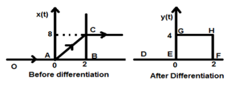
So our resulting signal y(t) can be written as;
$y(t) = \frac{dx(t)}{dt}$
$= \frac{d4[r(t)-r(t-2)]}{dt}$
$= 4[u(t)-u(t-2)]$
Now this signal is plotted finally, which is shown in the right hand side of the above figure.
DSP - Operations on Signals Integration
Integration of any signal means the summation of that signal under particular time domain to get a modified signal. Mathematically, this can be represented as −
$$x(t)\rightarrow y(t) = \int_{-\infty}^{t}x(t)dt$$Here also, in most of the cases we can do mathematical integration and find the resulted signal but direct integration in quick succession is possible for signals which are depicted in rectangular format graphically. Like differentiation, here also, we will refer a table to get the result quickly.
| Original Signal | Integrated Signal |
|---|---|
| 1 | impulse |
| Impulse | step |
| Step | Ramp |
Example
Let us consider a signal $x(t) = u(t)-u(t-3)$. It is shown in Fig-1 below. Clearly, we can see that it is a step signal. Now we will integrate it. Referring to the table, we know that integration of step signal yields ramp signal.
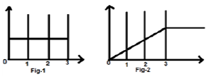
However, we will calculate it mathematically,
$y(t) = \int_{-\infty}^{t}x(t)dt$
$= \int_{-\infty}^{t}[u(t)-u(t-3)]dt$
$= \int_{-\infty}^{t}u(t)dt-\int_{-\infty}^{t}u(t-3)dt$
$= r(t)-r(t-3)$
The same is plotted as shown in fig-2,
DSP - Operations on Signals Convolution
The convolution of two signals in the time domain is equivalent to the multiplication of their representation in frequency domain. Mathematically, we can write the convolution of two signals as
$$y(t) = x_{1}(t)*x_{2}(t)$$ $$= \int_{-\infty}^{\infty}x_{1}(p).x_{2}(t-p)dp$$Steps for convolution
- Take signal x1(t) and put t = p there so that it will be x1(p).
- Take the signal x2(t) and do the step 1 and make it x2(p).
- Make the folding of the signal i.e. x2(-p).
- Do the time shifting of the above signal x2[-(p-t)]
- Then do the multiplication of both the signals. i.e. $x_{1}(p).x_{2}[−(p−t)]$
Example
Let us do the convolution of a step signal u(t) with its own kind.
$y(t) = u(t)*u(t)$
$= \int_{-\infty}^{\infty}[u(p).u[-(p-t)]dp$
Now this t can be greater than or less than zero, which are shown in below figures
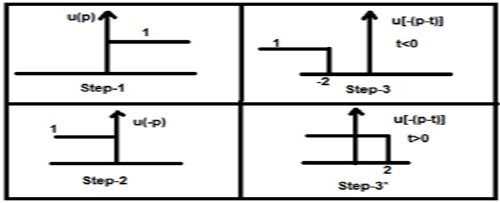
So, with the above case, the result arises with following possibilities
$y(t) = \begin{cases}0, & if\quad t<0\\\int_{0}^{t}1dt, & for\quad t>0\end{cases}$
$= \begin{cases}0, & if\quad t<0\\t, & t>0\end{cases} = r(t)$
Properties of Convolution
Commutative
It states that order of convolution does not matter, which can be shown mathematically as
$$x_{1}(t)*x_{2}(t) = x_{2}(t)*x_{1}(t)$$Associative
It states that order of convolution involving three signals, can be anything. Mathematically, it can be shown as;
$$x_{1}(t)*[x_{2}(t)*x_{3}(t)] = [x_{1}(t)*x_{2}(t)]*x_{3}(t)$$Distributive
Two signals can be added first, and then their convolution can be made to the third signal. This is equivalent to convolution of two signals individually with the third signal and added finally. Mathematically, this can be written as;
$$x_{1}(t)*[x_{2}(t)+x_{3}(t)] = [x_{1}(t)*x_{2}(t)+x_{1}(t)*x_{3}(t)]$$Area
If a signal is the result of convolution of two signals then the area of the signal is the multiplication of those individual signals. Mathematically this can be written
If $y(t) = x_{1}*x_{2}(t)$
Then, Area of y(t) = Area of x1(t) X Area of x2(t)
Scaling
If two signals are scaled to some unknown constant “a” and convolution is done then resultant signal will also be convoluted to same constant “a” and will be divided by that quantity as shown below.
If, $x_{1}(t)*x_{2}(t) = y(t)$
Then, $x_{1}(at)*x_{2}(at) = \frac{y(at)}{a}, a \ne 0$
Delay
Suppose a signal y(t) is a result from the convolution of two signals x1(t) and x2(t). If the two signals are delayed by time t1 and t2 respectively, then the resultant signal y(t) will be delayed by (t1+t2). Mathematically, it can be written as −
If, $x_{1}(t)*x_{2}(t) = y(t)$
Then, $x_{1}(t-t_{1})*x_{2}(t-t_{2}) = y[t-(t_{1}+t_{2})]$
Solved Examples
Example 1 − Find the convolution of the signals u(t-1) and u(t-2).
Solution − Given signals are u(t-1) and u(t-2). Their convolution can be done as shown below −
$y(t) = u(t-1)*u(t-2)$
$y(t) = \int_{-\infty}^{+\infty}[u(t-1).u(t-2)]dt$
$= r(t-1)+r(t-2)$
$= r(t-3)$
Example 2 − Find the convolution of two signals given by
$x_{1}(n) = \lbrace 3,-2, 2\rbrace $
$x_{2}(n) = \begin{cases}2, & 0\leq n\leq 4\\0, & x > elsewhere\end{cases}$
Solution −
x2(n) can be decoded as $x_{2}(n) = \lbrace 2,2,2,2,2\rbrace Originalfirst$
x1(n) is previously given $= \lbrace 3,-2,3\rbrace = 3-2Z^{-1}+2Z^{-2}$
Similarly, $x_{2}(z) = 2+2Z^{-1}+2Z^{-2}+2Z^{-3}+2Z^{-4}$
Resultant signal,
$X(Z) = X_{1}(Z)X_{2}(z)$
$= \lbrace 3-2Z^{-1}+2Z^{-2}\rbrace \times \lbrace 2+2Z^{-1}+2Z^{-2}+2Z^{-3}+2Z^{-4}\rbrace$
$= 6+2Z^{-1}+6Z^{-2}+6Z^{-3}+6Z^{-4}+6Z^{-5}$
Taking inverse Z-transformation of the above, we will get the resultant signal as
$x(n) = \lbrace 6,2,6,6,6,0,4\rbrace$ Origin at the first
Example 3 − Determine the convolution of following 2 signals −
$x(n) = \lbrace 2,1,0,1\rbrace$
$h(n) = \lbrace 1,2,3,1\rbrace$
Solution −
Taking the Z-transformation of the signals, we get,
$x(z) = 2+2Z^{-1}+2Z^{-3}$
And $h(n) = 1+2Z^{-1}+3Z^{-2}+Z^{-3}$
Now convolution of two signal means multiplication of their Z-transformations
That is $Y(Z) = X(Z) \times h(Z)$
$= \lbrace 2+2Z^{-1}+2Z^{-3}\rbrace \times \lbrace 1+2Z^{-1}+3Z^{-2}+Z^{-3}\rbrace$
$= \lbrace 2+5Z^{-1}+8Z^{-2}+6Z^{-3}+3Z^{-4}+3Z^{-5}+Z^{-6}\rbrace$
Taking the inverse Z-transformation, the resultant signal can be written as;
$y(n) = \lbrace 2,5,8,6,6,1 \rbrace Originalfirst$
Digital Signal Processing - Static Systems
Some systems have feedback and some do not. Those, which do not have feedback systems, their output depends only upon the present values of the input. Past value of the data is not present at that time. These types of systems are known as static systems. It does not depend upon future values too.
Since these systems do not have any past record, so they do not have any memory also. Therefore, we say all static systems are memory-less systems. Let us take an example to understand this concept much better.
Example
Let us verify whether the following systems are static systems or not.
- $y(t) = x(t)+x(t-1)$
- $y(t) = x(2t)$
- $y(t) = x = \sin [x(t)]$
a) $y(t) = x(t)+x(t-1)$
Here, x(t) is the present value. It has no relation with the past values of the time. So, it is a static system. However, in case of x(t-1), if we put t = 0, it will reduce to x(-1) which is a past value dependent. So, it is not static. Therefore here y(t) is not a static system.
b) $y(t) = x(2t)$
If we substitute t = 2, the result will be y(t) = x(4). Again, it is future value dependent. So, it is also not a static system.
c) $y(t) = x = \sin [x(t)]$
In this expression, we are dealing with sine function. The range of sine function lies within -1 to +1. So, whatever the values we substitute for x(t), we will get in between -1 to +1. Therefore, we can say it is not dependent upon any past or future values. Hence, it is a static system.
From the above examples, we can draw the following conclusions −
- Any system having time shifting is not static.
- Any system having amplitude shifting is also not static.
- Integration and differentiation cases are also not static.
Digital Signal Processing - Dynamic Systems
If a system depends upon the past and future value of the signal at any instant of the time then it is known as dynamic system. Unlike static systems, these are not memory less systems. They store past and future values. Therefore, they require some memory. Let us understand this theory better through some examples.
Examples
Find out whether the following systems are dynamic.
a) $y(t) = x(t+1)$
In this case if we put t = 1 in the equation, it will be converted to x(2), which is a future dependent value. Because here we are giving input as 1 but it is showing value for x(2). As it is a future dependent signal, so clearly it is a dynamic system.
b) $y(t) = Real[x(t)]$
$$= \frac{[x(t)+x(t)^*]}{2}$$In this case, whatever the value we will put it will show that time real value signal. It has no dependency on future or past values. Therefore, it is not a dynamic system rather it is a static system.
c) $y(t) = Even[x(t)]$
$$= \frac{[x(t)+x(-t)]}{2}$$Here, if we will substitute t = 1, one signal shows x(1) and another will show x(-1) which is a past value. Similarly, if we will put t = -1 then one signal will show x(-1) and another will show x(1) which is a future value. Therefore, clearly it is a case of Dynamic system.
d) $y(t) = \cos [x(t)]$
In this case, as the system is cosine function it has a certain domain of values which lies between -1 to +1. Therefore, whatever values we will put we will get the result within specified limit. Therefore, it is a static system
From the above examples, we can draw the following conclusions −
- All time shifting cases signals are dynamic signals.
- In case of time scaling too, all signals are dynamic signals.
- Integration cases signals are dynamic signals.
Digital Signal Processing - Causal Systems
Previously, we saw that the system needs to be independent from the future and past values to become static. In this case, the condition is almost same with little modification. Here, for the system to be causal, it should be independent from the future values only. That means past dependency will cause no problem for the system from becoming causal.
Causal systems are practically or physically realizable system. Let us consider some examples to understand this much better.
Examples
Let us consider the following signals.
a) $y(t) = x(t)$
Here, the signal is only dependent on the present values of x. For example if we substitute t = 3, the result will show for that instant of time only. Therefore, as it has no dependence on future value, we can call it a Causal system.
b) $y(t) = x(t-1)$
Here, the system depends on past values. For instance if we substitute t = 3, the expression will reduce to x(2), which is a past value against our input. At no instance, it depends upon future values. Therefore, this system is also a causal system.
c) $y(t) = x(t)+x(t+1)$
In this case, the system has two parts. The part x(t), as we have discussed earlier, depends only upon the present values. So, there is no issue with it. However, if we take the case of x(t+1), it clearly depends on the future values because if we put t = 1, the expression will reduce to x(2) which is future value. Therefore, it is not causal.
DSP - Non-Causal Systems
A non-causal system is just opposite to that of causal system. If a system depends upon the future values of the input at any instant of the time then the system is said to be non-causal system.
Examples
Let us take some examples and try to understand this in a better way.
a) $y(t) = x(t+1)$
We have already discussed this system in causal system too. For any input, it will reduce the system to its future value. For instance, if we put t = 2, it will reduce to x(3), which is a future value. Therefore, the system is Non-Causal.
b) $y(t) = x(t)+x(t+2)$
In this case, x(t) is purely a present value dependent function. We have already discussed that x(t+2) function is future dependent because for t = 3 it will give values for x(5). Therefore, it is Non-causal.
c) $y(t) = x(t-1)+x(t)$
In this system, it depends upon the present and past values of the given input. Whatever values we substitute, it will never show any future dependency. Clearly, it is not a non-causal system; rather it is a Causal system.
DSP - Anti-Causal Systems
An anti-causal system is just a little bit modified version of a non-causal system. The system depends upon the future values of the input only. It has no dependency either on present or on the past values.
Examples
Find out whether the following systems are anti-causal.
a) $y(t) = x(t)+x(t-1)$
The system has two sub-functions. One sub function x(t+1) depends on the future value of the input but another sub-function x(t) depends only on the present. As the system is dependent on the present value also in addition to future value, this system is not anti-causal.
b) $y(t) = x(t+3)$
If we analyze the above system, we can see that the system depends only on the future values of the system i.e. if we put t = 0, it will reduce to x(3), which is a future value. This system is a perfect example of anti-causal system.
Digital Signal Processing - Linear Systems
A linear system follows the laws of superposition. This law is necessary and sufficient condition to prove the linearity of the system. Apart from this, the system is a combination of two types of laws −
- Law of additivity
- Law of homogeneity
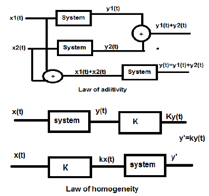
Both, the law of homogeneity and the law of additivity are shown in the above figures. However, there are some other conditions to check whether the system is linear or not.
The conditions are −
- The output should be zero for zero input.
- There should not be any non-linear operator present in the system.
Examples of non-linear operators −
(a) Trigonometric operators- Sin, Cos, Tan, Cot, Sec, Cosec etc.
(b) Exponential, logarithmic, modulus, square, Cube etc.
(c) sa(i/p) , Sinc (i/p) , Sqn (i/p) etc.
Either input x or output y should not have these non-linear operators.
Examples
Let us find out whether the following systems are linear.
a) $y(t) = x(t)+3$
This system is not a linear system because it violates the first condition. If we put input as zero, making x(t) = 0, then the output is not zero.
b) $y(t) = \sin tx(t)$
In this system, if we give input as zero, the output will become zero. Hence, the first condition is clearly satisfied. Again, there is no non-linear operator that has been applied on x(t). Hence, second condition is also satisfied. Therefore, the system is a linear system.
c) $y(t) = \sin (x(t))$
In the above system, first condition is satisfied because if we put x(t) = 0, the output will also be sin(0) = 0. However, the second condition is not satisfied, as there is a non-linear operator which operates x(t). Hence, the system is not linear.
DSP - Non-Linear Systems
If we want to define this system, we can say that the systems, which are not linear are non-linear systems. Clearly, all the conditions, which are being violated in the linear systems, should be satisfied in this case.
Conditions
The output should not be zero when input applied is zero.
Any non-linear operator can be applied on the either input or on the output to make the system non-linear.
Examples
To find out whether the given systems are linear or non-linear.
a) $y(t) = e^{x(t)}$
In the above system, the first condition is satisfied because if we make the input zero, the output is 1. In addition, exponential non-linear operator is applied to the input. Clearly, it is a case of Non-Linear system.
b) $y(t) = x(t+1)+x(t-1)$
The above type of system deals with both past and future values. However, if we will make its input zero, then none of its values exists. Therefore, we can say if the input is zero, then the time scaled and time shifted version of input will also be zero, which violates our first condition. Again, there is no non-linear operator present. Therefore, second condition is also violated. Clearly, this system is not a non-linear system; rather it is a linear system.
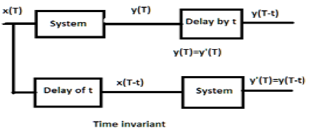
DSP - Time-Invariant Systems
For a time-invariant system, the output and input should be delayed by some time unit. Any delay provided in the input must be reflected in the output for a time invariant system.
Examples
a) $y(T) = x(2T)$
If the above expression, it is first passed through the system and then through the time delay (as shown in the upper part of the figure); then the output will become $x(2T-2t)$. Now, the same expression is passed through a time delay first and then through the system (as shown in the lower part of the figure). The output will become $x(2T-t)$.
Hence, the system is not a time-invariant system.
b) $y(T) = \sin [x(T)]$
If the signal is first passed through the system and then through the time delay process, the output be $\sin x(T-t)$. Similarly, if the system is passed through the time delay first then through the system then output will be $\sin x(T-t)$. We can see clearly that both the outputs are same. Hence, the system is time invariant.
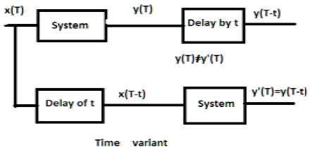
DSP - Time-Variant Systems
For a time variant system, also, output and input should be delayed by some time constant but the delay at the input should not reflect at the output. All time scaling cases are examples of time variant system. Similarly, when coefficient in the system relationship is a function of time, then also, the system is time variant.
Examples
a) $y(t) = x[\cos T]$
If the above signal is first passed through the system and then through the time delay, the output will be $x\cos (T-t)$. If it is passed through the time delay first and then through the system, it will be $x(\cos T-t)$. As the outputs are not same, the system is time variant.
b) $y(T) = \cos T.x(T)$
If the above expression is first passed through the system and then through the time delay, then the output will be $\cos(T-t)x(T-t)$. However, if the expression is passed through the time delay first and then through the system, the output will be $\cos T.x(T-t)$. As the outputs are not same, clearly the system is time variant.
Digital Signal Processing - Stable Systems
A stable system satisfies the BIBO (bounded input for bounded output) condition. Here, bounded means finite in amplitude. For a stable system, output should be bounded or finite, for finite or bounded input, at every instant of time.
Some examples of bounded inputs are functions of sine, cosine, DC, signum and unit step.
Examples
a) $y(t) = x(t)+10$
Here, for a definite bounded input, we can get definite bounded output i.e. if we put $x(t) = 2, y(t) = 12$ which is bounded in nature. Therefore, the system is stable.
b) $y(t) = \sin [x(t)]$
In the given expression, we know that sine functions have a definite boundary of values, which lies between -1 to +1. So, whatever values we will substitute at x(t), we will get the values within our boundary. Therefore, the system is stable.
Digital Signal Processing - Unstable Systems
Unstable systems do not satisfy the BIBO conditions. Therefore, for a bounded input, we cannot expect a bounded output in case of unstable systems.
Examples
a) $y(t) = tx(t)$
Here, for a finite input, we cannot expect a finite output. For example, if we will put $x(t) = 2 \Rightarrow y(t) = 2t$. This is not a finite value because we do not know the value of t. So, it can be ranged from anywhere. Therefore, this system is not stable. It is an unstable system.
b) $y(t) = \frac{x(t)}{\sin t}$
We have discussed earlier, that the sine function has a definite range from -1 to +1; but here, it is present in the denominator. So, in worst case scenario, if we put t = 0 and sine function becomes zero, then the whole system will tend to infinity. Therefore, this type of system is not at all stable. Obviously, this is an unstable system.
DSP - System Properties Solved Examples
Example 1 − Check whether $y(t) = x*(t)$ is linear or non-linear.
Solution − The function represents the conjugate of input. It can be verified by either first law of homogeneity and law of additivity or by the two rules. However, verifying through rules is lot easier, so we will go by that.
If the input to the system is zero, the output also tends to zero. Therefore, our first condition is satisfied. There is no non-linear operator used either at the input nor the output. Therefore, the system is Linear.
Example 2 − Check whether $y(t)=\begin{cases}x(t+1), & t > 0\\x(t-1), & t\leq 0\end{cases}$ is linear or non linear
Solution − Clearly, we can see that when time becomes less than or equal to zero the input becomes zero. So, we can say that at zero input the output is also zero and our first condition is satisfied.
Again, there is no non-linear operator used at the input nor at the output. Therefore, the system is Linear.
Example 3 − Check whether $y(t) = \sin t.x(t)$ is stable or not.
Solution − Suppose, we have taken the value of x(t) as 3. Here, sine function has been multiplied with it and maximum and minimum value of sine function varies between -1 to +1.
Therefore, the maximum and minimum value of the whole function will also vary between -3 and +3. Thus, the system is stable because here we are getting a bounded input for a bounded output.
DSP - Z-Transform Introduction
Discrete Time Fourier Transform(DTFT) exists for energy and power signals. Z-transform also exists for neither energy nor Power (NENP) type signal, up to a certain extent only. The replacement $z=e^{jw}$ is used for Z-transform to DTFT conversion only for absolutely summable signal.
So, the Z-transform of the discrete time signal x(n) in a power series can be written as −
$$X(z) = \sum_{n-\infty}^\infty x(n)Z^{-n}$$The above equation represents a two-sided Z-transform equation.
Generally, when a signal is Z-transformed, it can be represented as −
$$X(Z) = Z[x(n)]$$Or $x(n) \longleftrightarrow X(Z)$
If it is a continuous time signal, then Z-transforms are not needed because Laplace transformations are used. However, Discrete time signals can be analyzed through Z-transforms only.
Region of Convergence
Region of Convergence is the range of complex variable Z in the Z-plane. The Z- transformation of the signal is finite or convergent. So, ROC represents those set of values of Z, for which X(Z) has a finite value.
Properties of ROC
- ROC does not include any pole.
- For right-sided signal, ROC will be outside the circle in Z-plane.
- For left sided signal, ROC will be inside the circle in Z-plane.
- For stability, ROC includes unit circle in Z-plane.
- For Both sided signal, ROC is a ring in Z-plane.
- For finite-duration signal, ROC is entire Z-plane.
The Z-transform is uniquely characterized by −
- Expression of X(Z)
- ROC of X(Z)
Signals and their ROC
| x(n) | X(Z) | ROC |
|---|---|---|
| $\delta(n)$ | $1$ | Entire Z plane |
| $U(n)$ | $1/(1-Z^{-1})$ | Mod(Z)>1 |
| $a^nu(n)$ | $1/(1-aZ^{-1})$ | Mod(Z)>Mod(a) |
| $-a^nu(-n-1)$ | $1/(1-aZ^{-1})$ | Mod(Z)<Mod(a) |
| $na^nu(n)$ | $aZ^{-1}/(1-aZ^{-1})^2$ | Mod(Z)>Mod(a) |
| $-a^nu(-n-1)$ | $aZ^{-1}/(1-aZ^{-1})^2$ | Mod(Z)<Mod(a) |
| $U(n)\cos \omega n$ | $(Z^2-Z\cos \omega)/(Z^2-2Z \cos \omega +1)$ | Mod(Z)>1 |
| $U(n)\sin \omega n$ | $(Z\sin \omega)/(Z^2-2Z \cos \omega +1)$ | Mod(Z)>1 |
Example
Let us find the Z-transform and the ROC of a signal given as $x(n) = \lbrace 7,3,4,9,5\rbrace$, where origin of the series is at 3.
Solution − Applying the formula we have −
$X(z) = \sum_{n=-\infty}^\infty x(n)Z^{-n}$
$= \sum_{n=-1}^3 x(n)Z^{-n}$
$= x(-1)Z+x(0)+x(1)Z^{-1}+x(2)Z^{-2}+x(3)Z^{-3}$
$= 7Z+3+4Z^{-1}+9Z^{-2}+5Z^{-3}$
ROC is the entire Z-plane excluding Z = 0, ∞, -∞
DSP - Z-Transform Properties
In this chapter, we will understand the basic properties of Z-transforms.
Linearity
It states that when two or more individual discrete signals are multiplied by constants, their respective Z-transforms will also be multiplied by the same constants.
Mathematically,
$$a_1x_1(n)+a_2x_2(n) = a_1X_1(z)+a_2X_2(z)$$Proof − We know that,
$$X(Z) = \sum_{n=-\infty}^\infty x(n)Z^{-n}$$$= \sum_{n=-\infty}^\infty (a_1x_1(n)+a_2x_2(n))Z^{-n}$
$= a_1\sum_{n = -\infty}^\infty x_1(n)Z^{-n}+a_2\sum_{n = -\infty}^\infty x_2(n)Z^{-n}$
$= a_1X_1(z)+a_2X_2(z)$ (Hence Proved)
Here, the ROC is $ROC_1\bigcap ROC_2$.
Time Shifting
Time shifting property depicts how the change in the time domain in the discrete signal will affect the Z-domain, which can be written as;
$$x(n-n_0)\longleftrightarrow X(Z)Z^{-n}$$Or $x(n-1)\longleftrightarrow Z^{-1}X(Z)$
Proof −
Let $y(P) = X(P-K)$
$Y(z) = \sum_{p = -\infty}^\infty y(p)Z^{-p}$
$= \sum_{p = -\infty}^\infty (x(p-k))Z^{-p}$
Let s = p-k
$= \sum_{s = -\infty}^\infty x(s)Z^{-(s+k)}$
$= \sum_{s = -\infty}^\infty x(s)Z^{-s}Z^{-k}$
$= Z^{-k}[\sum_{s=-\infty}^\infty x(m)Z^{-s}]$
$= Z^{-k}X(Z)$ (Hence Proved)
Here, ROC can be written as Z = 0 (p>0) or Z = ∞(p<0)
Example
U(n) and U(n-1) can be plotted as follows
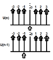
Z-transformation of U(n) cab be written as;
$\sum_{n = -\infty}^\infty [U(n)]Z^{-n} = 1$
Z-transformation of U(n-1) can be written as;
$\sum_{n = -\infty}^\infty [U(n-1)]Z^{-n} = Z^{-1}$
So here $x(n-n_0) = Z^{-n_0}X(Z)$ (Hence Proved)
Time Scaling
Time Scaling property tells us, what will be the Z-domain of the signal when the time is scaled in its discrete form, which can be written as;
$$a^nx(n) \longleftrightarrow X(a^{-1}Z)$$Proof −
Let $y(p) = a^{p}x(p)$
$Y(P) = \sum_{p=-\infty}^\infty y(p)Z^{-p}$
$= \sum_{p=-\infty}^\infty a^px(p)Z^{-p}$
$= \sum_{p=-\infty}^\infty x(p)[a^{-1}Z]^{-p}$
$= X(a^{-1}Z)$(Hence proved)
ROC: = Mod(ar1) < Mod(Z) < Mod(ar2) where Mod = Modulus
Example
Let us determine the Z-transformation of $x(n) = a^n \cos \omega n$ using Time scaling property.
Solution −
We already know that the Z-transformation of the signal $\cos (\omega n)$ is given by −
$$\sum_{n=-\infty}^\infty(\cos \omega n)Z^{-n} = (Z^2-Z \cos \omega)/(Z^2-2Z\cos \omega +1)$$
Now, applying Time scaling property, the Z-transformation of $a^n \cos \omega n$ can be written as;
$\sum_{n=-\infty}^\infty(a^n\cos \omega n)Z^{-n} = X(a^{-1}Z)$
$= [(a^{-1}Z)^2-(a^{-1}Z \cos \omega n)]/((a^{-1}Z)^2-2(a^{-1}Z \cos \omega n)+1)$
$= Z(Z-a \cos \omega)/(Z^2-2az \cos \omega+a^2)$
Successive Differentiation
Successive Differentiation property shows that Z-transform will take place when we differentiate the discrete signal in time domain, with respect to time. This is shown as below.
$$\frac{dx(n)}{dn} = (1-Z^{-1})X(Z)$$Proof −
Consider the LHS of the equation − $\frac{dx(n)}{dn}$
$$= \frac{[x(n)-x(n-1)]}{[n-(n-1)]}$$$= x(n)-X(n-1)$
$= x(Z)-Z^{-1}x(Z)$
$= (1-Z^{-1})x(Z)$ (Hence Proved)
ROC: R1< Mod (Z) <R2
Example
Let us find the Z-transform of a signal given by $x(n) = n^2u(n)$
By property we can write
$Zz[nU(n)] = -Z\frac{dZ[U(n)]}{dz}$
$= -Z\frac{d[\frac{Z}{Z-1}]}{dZ}$
$= Z/((Z-1)^2$
$= y(let)$
Now, Z[n.y] can be found out by again applying the property,
$Z(n,y) = -Z\frac{dy}{dz}$
$= -Z\frac{d[Z/(Z-1)^3]}{dz}$
$= Z(Z+1)/(Z-1)^2$
Convolution
This depicts the change in Z-domain of the system when a convolution takes place in the discrete signal form, which can be written as −
$x_1(n)*x_2(n) \longleftrightarrow X_1(Z).X_2(Z)$
Proof −
$X(Z) = \sum_{n = -\infty}^\infty x(n)Z^{-n}$
$= \sum_{n=-\infty}^\infty[\sum_{k = -\infty}^\infty x_1(k)x_2(n-k)]Z^{-n}$
$= \sum_{k = -\infty}^\infty x_1(k)[\sum_n^\infty x_2(n-k)Z^{-n}]$
$= \sum_{k = -\infty}^\infty x_1(k)[\sum_{n = -\infty}^\infty x_2(n-k)Z^{-(n-k)}Z^{-k}]$
Let n-k = l, then the above equation cab be written as −
$X(Z) = \sum_{k = -\infty}^\infty x_1(k)[Z^{-k}\sum_{l=-\infty}^\infty x_2(l)Z^{-l}]$
$= \sum_{k = -\infty}^\infty x_1(k)X_2(Z)Z^{-k}$
$= X_2(Z)\sum_{k = -\infty}^\infty x_1(Z)Z^{-k}$
$= X_1(Z).X_2(Z)$ (Hence Proved)
ROC:$ROC\bigcap ROC2$
Example
Let us find the convolution given by two signals
$x_1(n) = \lbrace 3,-2,2\rbrace$ ...(eq. 1)
$x_2(n) = \lbrace 2,0\leq 4\quad and\quad 0\quad elsewhere\rbrace$ ...(eq. 2)
Z-transformation of the first equation can be written as;
$\sum_{n = -\infty}^\infty x_1(n)Z^{-n}$
$= 3-2Z^{-1}+2Z^{-2}$
Z-transformation of the second signal can be written as;
$\sum_{n = -\infty}^\infty x_2(n)Z^{-n}$
$= 2+2Z^{-1}+2Z^{-2}+2Z^{-3}+2Z^{-4}$
So, the convolution of the above two signals is given by −
$X(Z) = [x_1(Z)^*x_2(Z)]$
$= [3-2Z^{-1}+2Z^{-2}]\times [2+2Z^{-1}+2Z^{-2}+2Z^{-3}+2Z^{-4}]$
$= 6+2Z^{-1}+6Z^{-2}+6Z^{-3}+...\quad...\quad...$
Taking the inverse Z-transformation we get,
$x(n) = \lbrace 6,2,6,6,6,0,4\rbrace$
Initial Value Theorem
If x(n) is a causal sequence, which has its Z-transformation as X(z), then the initial value theorem can be written as;
$X(n)(at\quad n = 0) = \lim_{z \to \infty} X(z)$
Proof − We know that,
$X(Z) = \sum_{n = 0} ^\infty x(n)Z^{-n}$
Expanding the above series, we get;
$= X(0)Z^0+X(1)Z^{-1}+X(2)Z^{-2}+...\quad...$
$= X(0)\times 1+X(1)Z^{-1}+X(2)Z^{-2}+...\quad...$
In the above case if Z → ∞ then $Z^{-n}\rightarrow 0$ (Because n>0)
Therefore, we can say;
$\lim_{z \to \infty}X(z) = X(0)$ (Hence Proved)
Final Value Theorem
Final Value Theorem states that if the Z-transform of a signal is represented as X(Z) and the poles are all inside the circle, then its final value is denoted as x(n) or X(∞) and can be written as −
$X(\infty) = \lim_{n \to \infty}X(n) = \lim_{z \to 1}[X(Z)(1-Z^{-1})]$
Conditions −
- It is applicable only for causal systems.
- $X(Z)(1-Z^{-1})$ should have poles inside the unit circle in Z-plane.
Proof − We know that
$Z^+[x(n+1)-x(n)] = \lim_{k \to \infty}\sum_{n=0}^kZ^{-n}[x(n+1)-x(n)]$
$\Rightarrow Z^+[x(n+1)]-Z^+[x(n)] = \lim_{k \to \infty}\sum_{n=0}^kZ^{-n}[x(n+1)-x(n)]$
$\Rightarrow Z[X(Z)^+-x(0)]-X(Z)^+ = \lim_{k \to \infty}\sum_{n = 0}^kZ^{-n}[x(n+1)-x(n)]$
Here, we can apply advanced property of one-sided Z-Transformation. So, the above equation can be re-written as;
$Z^+[x(n+1)] = Z[X(2)^+-x(0)Z^0] = Z[X(Z)^+-x(0)]$
Now putting z = 1 in the above equation, we can expand the above equation −
$\lim_{k \to \infty}{[x(1)-x(0)+x(6)-x(1)+x(3)-x(2)+...\quad...\quad...+x(x+1)-x(k)]}$
This can be formulated as;
$X(\infty) = \lim_{n \to \infty}X(n) = \lim_{z \to 1}[X(Z)(1-Z^{-1})]$(Hence Proved)
Example
Let us find the Initial and Final value of x(n) whose signal is given by
$X(Z) = 2+3Z^{-1}+4Z^{-2}$
Solution − Let us first, find the initial value of the signal by applying the theorem
$x(0) = \lim_{z \to \infty}X(Z)$
$= \lim_{z \to \infty}[2+3Z^{-1}+4Z^{-2}]$
$= 2+(\frac{3}{\infty})+(\frac{4}{\infty}) = 2$
Now let us find the Final value of signal applying the theorem
$x(\infty) = \lim_{z \to \infty}[(1-Z^{-1})X(Z)]$
$= \lim_{z \to \infty}[(1-Z^{-1})(2+3Z^{-1}+4Z^{-2})]$
$= \lim_{z \to \infty}[2+Z^{-1}+Z^{-2}-4Z^{-3}]$
$= 2+1+1-4 = 0$
Some other properties of Z-transform are listed below −
Differentiation in Frequency
It gives the change in Z-domain of the signal, when its discrete signal is differentiated with respect to time.
$nx(n)\longleftrightarrow -Z\frac{dX(z)}{dz}$
Its ROC can be written as;
$r_2< Mod(Z)< r_1$
Example
Let us find the value of x(n) through Differentiation in frequency, whose discrete signal in Z-domain is given by $x(n)\longleftrightarrow X(Z) = log(1+aZ^{-1})$
By property, we can write that
$nx(n)\longleftrightarrow -Z\frac{dx(Z)}{dz}$
$= -Z[\frac{-aZ^{-2}}{1+aZ^{-1}}]$
$= (aZ^{-1})/(1+aZ^{-1})$
$= 1-1/(1+aZ^{-1})$
$nx(n) = \delta(n)-(-a)^nu(n)$
$\Rightarrow x(n) = 1/n[\delta(n)-(-a)^nu(n)]$
Multiplication in Time
It gives the change in Z-domain of the signal when multiplication takes place at discrete signal level.
$x_1(n).x_2(n)\longleftrightarrow(\frac{1}{2\Pi j})[X1(Z)*X2(Z)]$
Conjugation in Time
This depicts the representation of conjugated discrete signal in Z-domain.
$X^*(n)\longleftrightarrow X^*(Z^*)$
DSP - Z-Transform Existence
A system, which has system function, can only be stable if all the poles lie inside the unit circle. First, we check whether the system is causal or not. If the system is Causal, then we go for its BIBO stability determination; where BIBO stability refers to the bounded input for bounded output condition.
This can be written as;
$Mod(X(Z))< \infty$
$= Mod(\sum x(n)Z^{-n})< \infty$
$= \sum Mod(x(n)Z^{-n})< \infty$
$= \sum Mod[x(n)(re^{jw})^{-n}]< 0$
$= \sum Mod[x(n)r^{-n}]Mod[e^{-jwn}]< \infty$
$= \sum_{n = -\infty}^\infty Mod[x(n)r^{-n}]< \infty$
The above equation shows the condition for existence of Z-transform.
However, the condition for existence of DTFT signal is
$$\sum_{n = -\infty}^\infty Mod(x(n)< \infty$$Example 1
Let us try to find out the Z-transform of the signal, which is given as
$x(n) = -(-0.5)^{-n}u(-n)+3^nu(n)$
$= -(-2)^nu(n)+3^nu(n)$
Solution − Here, for $-(-2)^nu(n)$ the ROC is Left sided and Z<2
For $3^nu(n)$ ROC is right sided and Z>3
Hence, here Z-transform of the signal will not exist because there is no common region.
Example 2
Let us try to find out the Z-transform of the signal given by
$x(n) = -2^nu(-n-1)+(0.5)^nu(n)$
Solution − Here, for $-2^nu(-n-1)$ ROC of the signal is Left sided and Z<2
For signal $(0.5)^nu(n)$ ROC is right sided and Z>0.5
So, the common ROC being formed as 0.5<Z<2
Therefore, Z-transform can be written as;
$X(Z) = \lbrace\frac{1}{1-2Z^{-1}}\rbrace+\lbrace\frac{1}{(1-0.5Z)^{-1}}\rbrace$
Example 3
Let us try to find out the Z-transform of the signal, which is given as $x(n) = 2^{r(n)}$
Solution − r(n) is the ramp signal. So the signal can be written as;
$x(n) = 2^{nu(n)}\lbrace 1, n<0 (u(n)=0)\quad and\quad2^n, n\geq 0(u(n) = 1)\rbrace$
$= u(-n-1)+2^nu(n)$
Here, for the signal $u(-n-1)$ and ROC Z<1 and for $2^nu(n)$ with ROC is Z>2.
So, Z-transformation of the signal will not exist.
Z -Transform for Causal System
Causal system can be defined as $h(n) = 0,n<0$. For causal system, ROC will be outside the circle in Z-plane.
$H(Z) = \displaystyle\sum\limits_{n = 0}^{\infty}h(n)Z^{-n}$
Expanding the above equation,
$H(Z) = h(0)+h(1)Z^{-1}+h(2)Z^{-2}+...\quad...\quad...$
$= N(Z)/D(Z)$
For causal systems, expansion of Transfer Function does not include positive powers of Z. For causal system, order of numerator cannot exceed order of denominator. This can be written as-
$\lim_{z \rightarrow \infty}H(Z) = h(0) = 0\quad or\quad Finite$
For stability of causal system, poles of Transfer function should be inside the unit circle in Z-plane.
Z-transform for Anti-causal System
Anti-causal system can be defined as $h(n) = 0, n\geq 0$ . For Anti causal system, poles of transfer function should lie outside unit circle in Z-plane. For anti-causal system, ROC will be inside the circle in Z-plane.
DSP - Z-Transform Inverse
If we want to analyze a system, which is already represented in frequency domain, as discrete time signal then we go for Inverse Z-transformation.
Mathematically, it can be represented as;
$$x(n) = Z^{-1}X(Z)$$where x(n) is the signal in time domain and X(Z) is the signal in frequency domain.
If we want to represent the above equation in integral format then we can write it as
$$x(n) = (\frac{1}{2\Pi j})\oint X(Z)Z^{-1}dz$$Here, the integral is over a closed path C. This path is within the ROC of the x(z) and it does contain the origin.
Methods to Find Inverse Z-Transform
When the analysis is needed in discrete format, we convert the frequency domain signal back into discrete format through inverse Z-transformation. We follow the following four ways to determine the inverse Z-transformation.
- Long Division Method
- Partial Fraction expansion method
- Residue or Contour integral method
Long Division Method
In this method, the Z-transform of the signal x (z) can be represented as the ratio of polynomial as shown below;
$$x(z)=N(Z)/D(Z)$$Now, if we go on dividing the numerator by denominator, then we will get a series as shown below
$$X(z) = x(0)+x(1)Z^{-1}+x(2)Z^{-2}+...\quad...\quad...$$The above sequence represents the series of inverse Z-transform of the given signal (for n≥0) and the above system is causal.
However for n<0 the series can be written as;
$$x(z) = x(-1)Z^1+x(-2)Z^2+x(-3)Z^3+...\quad...\quad...$$Partial Fraction Expansion Method
Here also the signal is expressed first in N (z)/D (z) form.
If it is a rational fraction it will be represented as follows;
$x(z) = b_0+b_1Z^{-1}+b_2Z^{-2}+...\quad...\quad...+b_mZ^{-m})/(a_0+a_1Z^{-1}+a_2Z^{-2}+...\quad...\quad...+a_nZ^{-N})$
The above one is improper when m<n and an≠0
If the ratio is not proper (i.e. Improper), then we have to convert it to the proper form to solve it.
Residue or Contour Integral Method
In this method, we obtain inverse Z-transform x(n) by summing residues of $[x(z)Z^{n-1}]$ at all poles. Mathematically, this may be expressed as
$$x(n) = \displaystyle\sum\limits_{all\quad poles\quad X(z)}residues\quad of[x(z)Z^{n-1}]$$Here, the residue for any pole of order m at $z = \beta$ is
$$Residues = \frac{1}{(m-1)!}\lim_{Z \rightarrow \beta}\lbrace \frac{d^{m-1}}{dZ^{m-1}}\lbrace (z-\beta)^mX(z)Z^{n-1}\rbrace$$DSP - Z-Transform Solved Examples
Example 1
Find the response of the system $s(n+2)-3s(n+1)+2s(n) = \delta (n)$, when all the initial conditions are zero.
Solution − Taking Z-transform on both the sides of the above equation, we get
$$S(z)Z^2-3S(z)Z^1+2S(z) = 1$$$\Rightarrow S(z)\lbrace Z^2-3Z+2\rbrace = 1$
$\Rightarrow S(z) = \frac{1}{\lbrace z^2-3z+2\rbrace}=\frac{1}{(z-2)(z-1)} = \frac{\alpha _1}{z-2}+\frac{\alpha _2}{z-1}$
$\Rightarrow S(z) = \frac{1}{z-2}-\frac{1}{z-1}$
Taking the inverse Z-transform of the above equation, we get
$S(n) = Z^{-1}[\frac{1}{Z-2}]-Z^{-1}[\frac{1}{Z-1}]$
$= 2^{n-1}-1^{n-1} = -1+2^{n-1}$
Example 2
Find the system function H(z) and unit sample response h(n) of the system whose difference equation is described as under
$y(n) = \frac{1}{2}y(n-1)+2x(n)$
where, y(n) and x(n) are the output and input of the system, respectively.
Solution − Taking the Z-transform of the above difference equation, we get
$y(z) = \frac{1}{2}Z^{-1}Y(Z)+2X(z)$
$= Y(Z)[1-\frac{1}{2}Z^{-1}] = 2X(Z)$
$= H(Z) = \frac{Y(Z)}{X(Z)} = \frac{2}{[1-\frac{1}{2}Z^{-1}]}$
This system has a pole at $Z = \frac{1}{2}$ and $Z = 0$ and $H(Z) = \frac{2}{[1-\frac{1}{2}Z^{-1}]}$
Hence, taking the inverse Z-transform of the above, we get
$h(n) = 2(\frac{1}{2})^nU(n)$
Example 3
Determine Y(z),n≥0 in the following case −
$y(n)+\frac{1}{2}y(n-1)-\frac{1}{4}y(n-2) = 0\quad given\quad y(-1) = y(-2) = 1$
Solution − Applying the Z-transform to the above equation, we get
$Y(Z)+\frac{1}{2}[Z^{-1}Y(Z)+Y(-1)]-\frac{1}{4}[Z^{-2}Y(Z)+Z^{-1}Y(-1)+4(-2)] = 0$
$\Rightarrow Y(Z)+\frac{1}{2Z}Y(Z)+\frac{1}{2}-\frac{1}{4Z^2}Y(Z)-\frac{1}{4Z}-\frac{1}{4} = 0$
$\Rightarrow Y(Z)[1+\frac{1}{2Z}-\frac{1}{4Z^2}] =\frac{1}{4Z}-\frac{1}{2}$
$\Rightarrow Y(Z)[\frac{4Z^2+2Z-1}{4Z^2}] = \frac{1-2Z}{4Z}$
$\Rightarrow Y(Z) = \frac{Z(1-2Z)}{4Z^2+2Z-1}$
Digital Signal Processing - DFT Introduction
Like continuous time signal Fourier transform, discrete time Fourier Transform can be used to represent a discrete sequence into its equivalent frequency domain representation and LTI discrete time system and develop various computational algorithms.
X (jω) in continuous F.T, is a continuous function of x(n). However, DFT deals with representing x(n) with samples of its spectrum X(ω). Hence, this mathematical tool carries much importance computationally in convenient representation. Both, periodic and non-periodic sequences can be processed through this tool. The periodic sequences need to be sampled by extending the period to infinity.
Frequency Domain Sampling
From the introduction, it is clear that we need to know how to proceed through frequency domain sampling i.e. sampling X(ω). Hence, the relationship between sampled Fourier transform and DFT is established in the following manner.
Similarly, periodic sequences can fit to this tool by extending the period N to infinity.
Let an Non periodic sequence be, $X(n) = \lim_{N \to \infty}x_N(n)$
Defining its Fourier transform,
$X(\omega ) = \sum_{n=-\infty}^\infty x(n)e^{-jwn}X(K\delta \omega)$
Here, X(ω) is sampled periodically, at every δω radian interval.
As X(ω) is periodic in 2π radians, we require samples only in fundamental range. The samples are taken after equidistant intervals in the frequency range 0≤ω≤2π. Spacing between equivalent intervals is $\delta \omega = \frac{2\pi }{N}k$ radian.
Now evaluating, $\omega = \frac{2\pi}{N}k$
$X(\frac{2\pi}{N}k) = \sum_{n = -\infty}^\infty x(n)e^{-j2\pi nk/N},$ ...eq(2)
where k=0,1,……N-1
After subdividing the above, and interchanging the order of summation
$X(\frac{2\pi}{N}k) = \displaystyle\sum\limits_{n = 0}^{N-1}[\displaystyle\sum\limits_{l = -\infty}^\infty x(n-Nl)]e^{-j2\pi nk/N}$ ...eq(3)
$\sum_{l=-\infty}^\infty x(n-Nl) = x_p(n) = a\quad periodic\quad function\quad of\quad period\quad N\quad and\quad its\quad fourier\quad series\quad = \sum_{k = 0}^{N-1}C_ke^{j2\pi nk/N}$
where, n = 0,1,…..,N-1; ‘p’- stands for periodic entity or function
The Fourier coefficients are,
$C_k = \frac{1}{N}\sum_{n = 0}^{N-1}x_p(n)e^{-j2\pi nk/N}$k=0,1,…,N-1...eq(4)
Comparing equations 3 and 4, we get ;
$NC_k = X(\frac{2\pi}{N}k)$ k=0,1,…,N-1...eq(5)
$NC_k = X(\frac{2\pi}{N}k) = X(e^{jw}) = \displaystyle\sum\limits_{n = -\infty}^\infty x_p(n)e^{-j2\pi nk/N}$...eq(6)
From Fourier series expansion,
$x_p(n) = \frac{1}{N}\displaystyle\sum\limits_{k = 0}^{N-1}NC_ke^{j2\pi nk/N} = \frac{1}{N}\sum_{k = 0}^{N-1}X(\frac{2\pi}{N}k)e^{j2\pi nk/N}$...eq(7)
Where n=0,1,…,N-1
Here, we got the periodic signal from X(ω). $x(n)$ can be extracted from $x_p(n)$ only, if there is no aliasing in the time domain. $N\geq L$
N = period of $x_p(n)$ L= period of $x(n)$
$x(n) = \begin{cases}x_p(n), & 0\leq n\leq N-1\\0, & Otherwise\end{cases}$
The mapping is achieved in this manner.
Properties of DFT
Linearity
It states that the DFT of a combination of signals is equal to the sum of DFT of individual signals. Let us take two signals x1(n) and x2(n), whose DFT s are X1(ω) and X2(ω) respectively. So, if
$x_1(n)\rightarrow X_1(\omega)$and$x_2(n)\rightarrow X_2(\omega)$
Then $ax_1(n)+bx_2(n)\rightarrow aX_1(\omega)+bX_2(\omega)$
where a and b are constants.
Symmetry
The symmetry properties of DFT can be derived in a similar way as we derived DTFT symmetry properties. We know that DFT of sequence x(n) is denoted by X(K). Now, if x(n) and X(K) are complex valued sequence, then it can be represented as under
$x(n) = x_R(n)+jx_1(n),0\leq n\leq N-1$
And $X(K) = X_R(K)+jX_1(K),0\leq K\leq N-1$
Duality Property
Let us consider a signal x(n), whose DFT is given as X(K). Let the finite duration sequence be X(N). Then according to duality theorem,
If, $x(n)\longleftrightarrow X(K)$
Then, $X(N)\longleftrightarrow Nx[((-k))_N]$
So, by using this theorem if we know DFT, we can easily find the finite duration sequence.
Complex Conjugate Properties
Suppose, there is a signal x(n), whose DFT is also known to us as X(K). Now, if the complex conjugate of the signal is given as x*(n), then we can easily find the DFT without doing much calculation by using the theorem shown below.
If, $x(n)\longleftrightarrow X(K)$
Then, $x*(n)\longleftrightarrow X*((K))_N = X*(N-K)$
Circular Frequency Shift
The multiplication of the sequence x(n) with the complex exponential sequence $e^{j2\Pi kn/N}$ is equivalent to the circular shift of the DFT by L units in frequency. This is the dual to the circular time shifting property.
If, $x(n)\longleftrightarrow X(K)$
Then, $x(n)e^{j2\Pi Kn/N}\longleftrightarrow X((K-L))_N$
Multiplication of Two Sequence
If there are two signal x1(n) and x2(n) and their respective DFTs are X1(k) and X2(K), then multiplication of signals in time sequence corresponds to circular convolution of their DFTs.
If, $x_1(n)\longleftrightarrow X_1(K)\quad\&\quad x_2(n)\longleftrightarrow X_2(K)$
Then, $x_1(n)\times x_2(n)\longleftrightarrow X_1(K)© X_2(K)$
Parseval’s Theorem
For complex valued sequences x(n) and y(n), in general
If, $x(n)\longleftrightarrow X(K)\quad \&\quad y(n)\longleftrightarrow Y(K)$
Then, $\sum_{n = 0}^{N-1}x(n)y^*(n) = \frac{1}{N}\sum_{k = 0}^{N-1}X(K)Y^*(K)$
DSP - DFT Time Frequency Transform
We know that when $\omega = 2\pi K/N$ and $N\rightarrow \infty,\omega$ becomes a continuous variable and limits summation become $-\infty$ to $+\infty$.
Therefore,
$$NC_k = X(\frac{2\pi}{N}k) = X(e^{j\omega}) = \displaystyle\sum\limits_{n = -\infty}^\infty x(n)e^{\frac{-j2\pi nk}{N}} = \displaystyle\sum\limits_{n = -\infty}^\infty x(n)e^{-j\omega n}$$Discrete Time Fourier Transform (DTFT)
We know that, $X(e^{j\omega}) = \sum_{n = -\infty}^\infty x(n)e^{-j\omega n}$
Where, $X(e^{j\omega})$ is continuous and periodic in ω and with period 2π.…eq(1)
Now,
$x_p(n) = \sum_{k = 0}^{N-1}NC_ke^{j2 \pi nk/N}$ … From Fourier series
$x_p(n) = \frac{1}{2\pi}\sum_{k=0}^{N-1}NC_ke^{j2\pi nk/N}\times \frac{2\pi}{N}$
ω becomes continuous and $\frac{2\pi}{N}\rightarrow d\omega$, because of the reasons cited above.
$x(n) = \frac{1}{2\pi}\int_{n = 0}^{2\pi}X(e^{j\omega})e^{j\omega n}d\omega$…eq(2)
Inverse Discrete Time Fourier Transform
Symbolically,
$x(n)\Longleftrightarrow x(e^{j\omega})$(The Fourier Transform pair)
Necessary and sufficient condition for existence of Discrete Time Fourier Transform for a non-periodic sequence x(n) is absolute summable.
i.e.$\sum_{n = -\infty}^\infty|x(n)|<\infty$
Properties of DTFT
Linearity : $a_1x_1(n)+a_2x_2(n)\Leftrightarrow a_1X_1(e^{j\omega})+a_2X_2(e^{j\omega})$
Time shifting − $x(n-k)\Leftrightarrow e^{-j\omega k}.X(e^{j\omega})$
Time Reversal − $x(-n)\Leftrightarrow X(e^{-j\omega})$
Frequency shifting − $e^{j\omega _0n}x(n)\Leftrightarrow X(e^{j(\omega -\omega _0)})$
Differentiation frequency domain − $nx(n) = j\frac{d}{d\omega}X(e^{j\omega})$
Convolution − $x_1(n)*x_2(n)\Leftrightarrow X_1(e^{j\omega})\times X_2(e^{j\omega})$
Multiplication − $x_1(n)\times x_2(n)\Leftrightarrow X_1(e^{j\omega})*X_2(e^{j\omega})$
Co-relation − $y_{x_1\times x_2}(l)\Leftrightarrow X_1(e^{j\omega})\times X_2(e^{j\omega})$
Modulation theorem − $x(n)\cos \omega _0n = \frac{1}{2}[X_1(e^{j(\omega +\omega _0})*X_2(e^{jw})$
Symmetry −$x^*(n)\Leftrightarrow X^*(e^{-j\omega})$ ;
$x^*(-n)\Leftrightarrow X^*(e^{j\omega})$ ;
$Real[x(n)]\Leftrightarrow X_{even}(e^{j\omega})$ ;
$Imag[x(n)]\Leftrightarrow X_{odd}(e^{j\omega})$ ;
$x_{even}(n)\Leftrightarrow Real[x(e^{j\omega})]$ ;
$x_{odd}(n)\Leftrightarrow Imag[x(e^{j\omega})]$ ;
Parseval’s theorem − $\sum_{-\infty}^\infty|x_1(n)|^2 = \frac{1}{2\pi}\int_{-\pi}^{\pi}|X_1(e^{j\omega})|^2d\omega$
Earlier, we studied sampling in frequency domain. With that basic knowledge, we sample $X(e^{j\omega})$ in frequency domain, so that a convenient digital analysis can be done from that sampled data. Hence, DFT is sampled in both time and frequency domain. With the assumption $x(n) = x_p(n)$
Hence, DFT is given by −
$X(k) = DFT[x(n)] = X(\frac{2\pi}{N}k) = \displaystyle\sum\limits_{n = 0}^{N-1}x(n)e^{-\frac{j2\pi nk}{N}}$,k=0,1,….,N−1…eq(3)
And IDFT is given by −
$X(n) = IDFT[X(k)] = \frac{1}{N}\sum_{k = 0}^{N-1}X(k)e^{\frac{j2\pi nk}{N}}$,n=0,1,….,N−1…eq(4)
$\therefore x(n)\Leftrightarrow X(k)$
Twiddle Factor
It is denoted as $W_N$ and defined as $W_N = e^{-j2\pi /N}$ . Its magnitude is always maintained at unity. Phase of $W_N = -2\pi /N$ . It is a vector on unit circle and is used for computational convenience. Mathematically, it can be shown as −
$W_N^r = W_N^{r\pm N} = W_N^{r\pm 2N} = ...$
It is function of r and period N.
Consider N = 8, r = 0,1,2,3,….14,15,16,….
$\Longleftrightarrow W_8^0 = W_8^8 = W_8^{16} = ... = ... = W_8^{32} = ... =1= 1\angle 0$
$W_8^1 = W_8^9 = W_8^{17} = ... = ... = W_8^{33} = ... =\frac{1}{\sqrt 2}= j\frac{1}{\sqrt 2} = 1\angle-\frac{\pi}{4}$
Linear Transformation
Let us understand Linear Transformation −
We know that,
$DFT(k) = DFT[x(n)] = X(\frac{2\pi}{N}k) = \sum_{n = 0}^{N-1}x(n).W_n^{-nk};\quad k = 0,1,….,N−1$
$x(n) = IDFT[X(k)] = \frac{1}{N}\sum_{k = 0}^{N-1}X(k).W_N^{-nk};\quad n = 0,1,….,N−1$
Note − Computation of DFT can be performed with N2 complex multiplication and N(N-1) complex addition.
$x_N = \begin{bmatrix}x(0)\\x(1)\\.\\.\\x(N-1) \end{bmatrix}\quad N\quad point\quad vector\quad of\quad signal\quad x_N$
$X_N = \begin{bmatrix}X(0)\\X(1)\\.\\.\\X(N-1) \end{bmatrix}\quad N\quad point\quad vector\quad of\quad signal\quad X_N$
$\begin{bmatrix}1 & 1 & 1 & ... & ... & 1\\1 & W_N & W_N^2 & ... & ... & W_N^{N-1}\\. & W_N^2 & W_N^4 & ... & ... & W_N^{2(N-1)}\\.\\1 & W_N^{N-1} & W_N^{2(N-1)} & ... & ... & W_N^{(N-1)(N-1)} \end{bmatrix}$
N - point DFT in matrix term is given by - $X_N = W_Nx_N$
$W_N\longmapsto$ Matrix of linear transformation
$Now,\quad x_N = W_N^{-1}X_N$
IDFT in Matrix form is given by
$$x_N = \frac{1}{N}W_N^*X_N$$Comparing both the expressions of $x_N,\quad W_N^{-1} = \frac{1}{N}W_N^*$ and $W_N\times W_N^* = N[I]_{N\times N}$
Therefore, $W_N$ is a linear transformation matrix, an orthogonal (unitary) matrix.
From periodic property of $W_N$ and from its symmetric property, it can be concluded that, $W_N^{k+N/2} = -W_N^k$
Circular Symmetry
N-point DFT of a finite duration x(n) of length N≤L, is equivalent to the N-point DFT of periodic extension of x(n), i.e. $x_p(n)$ of period N. and $x_p(n) = \sum_{l = -\infty}^\infty x(n-Nl)$ . Now, if we shift the sequence, which is a periodic sequence by k units to the right, another periodic sequence is obtained. This is known as Circular shift and this is given by,
$$x_p^\prime (n) = x_p(n-k) = \sum_{l = -\infty}^\infty x(n-k-Nl)$$The new finite sequence can be represented as
$$x_p^\prime (n) = \begin{cases}x_p^\prime(n), & 0\leq n\leq N-1\\0 & Otherwise\end{cases}$$Example − Let x(n)= {1,2,4,3}, N = 4,
$x_p^\prime (n) = x(n-k,modulo\quad N)\equiv x((n-k))_N\quad;ex-if\quad k=2i.e\quad 2\quad unit\quad right\quad shift\quad and\quad N = 4,$
Assumed clockwise direction as positive direction.
We got, $x\prime(n) = x((n-2))_4$
$x\prime(0) = x((-2))_4 = x(2) = 4$
$x\prime(1) = x((-1))_4 = x(3) = 3$
$x\prime(2) = x((-2))_4 = x(0) = 1$
$x\prime(3) = x((1))_4 = x(1) = 2$
Conclusion − Circular shift of N-point sequence is equivalent to a linear shift of its periodic extension and vice versa.
Circularly even sequence − $x(N-n) = x(n),\quad 1\leq n\leq N-1$
$i.e.x_p(n) = x_p(-n) = x_p(N-n)$
Conjugate even −$x_p(n) = x_p^*(N-n)$
Circularly odd sequence − $x(N-n) = -x(n),\quad 1\leq n\leq N-1$
$i.e.x_p(n) = -x_p(-n) = -x_p(N-n)$
Conjugate odd − $x_p(n) = -x_p^*(N-n)$
Now, $x_p(n) = x_{pe}+x_{po}(n)$, where,
$x_{pe}(n) = \frac{1}{2}[x_p(n)+x_p^*(N-n)]$
$x_{po}(n) = \frac{1}{2}[x_p(n)-x_p^*(N-n)]$
For any real signal x(n),$X(k) = X^*(N-k)$
$X_R(k) = X_R(N-k)$
$X_l(k) = -X_l(N-k)$
$\angle X(k) = -\angle X(N-K)$
Time reversal − reversing sample about the 0th sample. This is given as;
$x((-n))_N = x(N-n),\quad 0\leq n\leq N-1$
Time reversal is plotting samples of sequence, in clockwise direction i.e. assumed negative direction.
Some Other Important Properties
Other important IDFT properties $x(n)\longleftrightarrow X(k)$
Time reversal − $x((-n))_N = x(N-n)\longleftrightarrow X((-k))_N = X(N-k)$
Circular time shift − $x((n-l))_N \longleftrightarrow X(k)e^{j2\pi lk/N}$
Circular frequency shift − $x(n)e^{j2\pi ln/N} \longleftrightarrow X((k-l))_N$
Complex conjugate properties −
$x^*(n)\longleftrightarrow X^*((-k))_N = X^*(N-k)\quad and$
$x^*((-n))_N = x^*(N-n)\longleftrightarrow X^*(-k)$
Multiplication of two sequence −
$x_1(n)\longleftrightarrow X_1(k)\quad and\quad x_2(n)\longleftrightarrow X_2(k)$
$\therefore x_1(n)x_2(n)\longleftrightarrow X_1(k)\quadⓃ X_2(k)$
Circular convolution − and multiplication of two DFT
$x_1(k)\quad Ⓝ x_2(k) =\sum_{k = 0}^{N-1}x_1(n).x_2((m-n))_n,\quad m = 0,1,2,... .,N-1 $
$x_1(k)\quad Ⓝ x_2(k)\longleftrightarrow X_1(k).X_2(k)$
Circular correlation − If $x(n)\longleftrightarrow X(k)$ and $y(n)\longleftrightarrow Y(k)$ , then there exists a cross correlation sequence denoted as $\bar Y_{xy}$ such that $\bar Y_{xy}(l) = \sum_{n = 0}^{N-1}x(n)y^*((n-l))_N = X(k).Y^*(k)$
Parseval’s Theorem − If $x(n)\longleftrightarrow X(k)$ and $y(n)\longleftrightarrow Y(k)$;
$\displaystyle\sum\limits_{n = 0}^{N-1}x(n)y^*(n) = \frac{1}{N}\displaystyle\sum\limits_{n =0}^{N-1}X(k).Y^*(k)$
DSP - DFT Circular Convolution
Let us take two finite duration sequences x1(n) and x2(n), having integer length as N. Their DFTs are X1(K) and X2(K) respectively, which is shown below −
$$X_1(K) = \sum_{n = 0}^{N-1}x_1(n)e^{\frac{j2\Pi kn}{N}}\quad k = 0,1,2...N-1$$ $$X_2(K) = \sum_{n = 0}^{N-1}x_2(n)e^{\frac{j2\Pi kn}{N}}\quad k = 0,1,2...N-1$$Now, we will try to find the DFT of another sequence x3(n), which is given as X3(K)
$X_3(K) = X_1(K)\times X_2(K)$
By taking the IDFT of the above we get
$x_3(n) = \frac{1}{N}\displaystyle\sum\limits_{n = 0}^{N-1}X_3(K)e^{\frac{j2\Pi kn}{N}}$
After solving the above equation, finally, we get
$x_3(n) = \displaystyle\sum\limits_{m = 0}^{N-1}x_1(m)x_2[((n-m))_N]\quad m = 0,1,2...N-1$
| Comparison points | Linear Convolution | Circular Convolution |
|---|---|---|
| Shifting | Linear shifting | Circular shifting |
| Samples in the convolution result | $N_1+N_2−1$ | $Max(N_1,N_2)$ |
| Finding response of a filter | Possible | Possible with zero padding |
Methods of Circular Convolution
Generally, there are two methods, which are adopted to perform circular convolution and they are −
- Concentric circle method,
- Matrix multiplication method.
Concentric Circle Method
Let $x_1(n)$ and $x_2(n)$ be two given sequences. The steps followed for circular convolution of $x_1(n)$ and $x_2(n)$ are
Take two concentric circles. Plot N samples of $x_1(n)$ on the circumference of the outer circle (maintaining equal distance successive points) in anti-clockwise direction.
For plotting $x_2(n)$, plot N samples of $x_2(n)$ in clockwise direction on the inner circle, starting sample placed at the same point as 0th sample of $x_1(n)$
Multiply corresponding samples on the two circles and add them to get output.
Rotate the inner circle anti-clockwise with one sample at a time.
Matrix Multiplication Method
Matrix method represents the two given sequence $x_1(n)$ and $x_2(n)$ in matrix form.
One of the given sequences is repeated via circular shift of one sample at a time to form a N X N matrix.
The other sequence is represented as column matrix.
The multiplication of two matrices give the result of circular convolution.
DSP - DFT Linear Filtering
DFT provides an alternative approach to time domain convolution. It can be used to perform linear filtering in frequency domain.
Thus,$Y(\omega) = X(\omega).H(\omega)\longleftrightarrow y(n)$.
The problem in this frequency domain approach is that $Y(\omega)$, $X(\omega)$ and $H(\omega)$ are continuous function of ω, which is not fruitful for digital computation on computers. However, DFT provides sampled version of these waveforms to solve the purpose.
The advantage is that, having knowledge of faster DFT techniques likes of FFT, a computationally higher efficient algorithm can be developed for digital computer computation in comparison with time domain approach.
Consider a finite duration sequence, $[x(n) = 0,\quad for,n<0\quad and\quad n\geq L]$ (generalized equation), excites a linear filter with impulse response $[h(n) = 0,\quad forn<0\quad and\quad n\geq M]$.
$$x(n)y(n)$$ $$output = y(n) = \sum_{k = 0}^{M-1}h(k).x(n-k)$$From the convolution analysis, it is clear that, the duration of y(n) is L+M−1.
In frequency domain,
$$Y(\omega) = X(\omega).H(\omega)$$Now, $Y(\omega)$ is a continuous function of ω and it is sampled at a set of discrete frequencies with number of distinct samples which must be equal to or exceeds $L+M-1$.
$$DFT\quad size = N\geq L+M-1$$With $\omega = \frac{2\pi}{N}k$,
$Y(\omega) = X(k).H(k)$, where k=0,1,….,N-1
Where, X(k) and H(k) are N-point DFTs of x(n) and h(n) respectively. $x(n)\& h(n)$ are padded with zeros up to the length N. It will not distort the continuous spectra $X(\omega)$ and $H(\omega)$. Since $N\geq L+M-1$, N-point DFT of output sequence y(n) is sufficient to represent y(n) in frequency domain and these facts infer that the multiplication of N-point DFTs of X(k) and H(k), followed by the computation of N-point IDFT must yield y(n).
This implies, N-point circular convolution of x(n) and H(n) with zero padding, equals to linear convolution of x(n) and h(n).
Thus, DFT can be used for linear filtering.
Caution − N should always be greater than or equal to $L+M-1$. Otherwise, aliasing effect would corrupt the output sequence.
DSP - DFT Sectional Convolution
Suppose, the input sequence x(n) of long duration is to be processed with a system having finite duration impulse response by convolving the two sequences. Since, the linear filtering performed via DFT involves operation on a fixed size data block, the input sequence is divided into different fixed size data block before processing.
The successive blocks are then processed one at a time and the results are combined to produce the net result.
As the convolution is performed by dividing the long input sequence into different fixed size sections, it is called sectioned convolution. A long input sequence is segmented to fixed size blocks, prior to FIR filter processing.
Two methods are used to evaluate the discrete convolution −
Overlap-save method
Overlap-add method
Overlap Save Method
Overlap–save is the traditional name for an efficient way to evaluate the discrete convolution between a very long signal x(n) and a finite impulse response (FIR) filter h(n). Given below are the steps of Overlap save method −
Let the length of input data block = N = L+M-1. Therefore, DFT and IDFT length = N. Each data block carries M-1 data points of previous block followed by L new data points to form a data sequence of length N = L+M-1.
First, N-point DFT is computed for each data block.
By appending (L-1) zeros, the impulse response of FIR filter is increased in length and N point DFT is calculated and stored.
Multiplication of two N-point DFTs H(k) and Xm(k) : Y′m(k) = H(k).Xm(k), where K=0,1,2,…N-1
Then, IDFT[Y′m((k)] = y′((n) = [y′m(0), y′m(1), y′m(2),.......y′m(M-1), y′m(M),.......y′m(N-1)]
(here, N-1 = L+M-2)
First M-1 points are corrupted due to aliasing and hence, they are discarded because the data record is of length N.
The last L points are exactly same as a result of convolution, so
y′m (n) = ym(n) where n = M, M+1,….N-1
To avoid aliasing, the last M-1 elements of each data record are saved and these points carry forward to the subsequent record and become 1st M-1 elements.
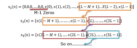
Result of IDFT, where first M-1 Points are avoided, to nullify aliasing and remaining L points constitute desired result as that of a linear convolution.
Overlap Add Method
Given below are the steps to find out the discrete convolution using Overlap method −
Let the input data block size be L. Therefore, the size of DFT and IDFT: N = L+M-1
Each data block is appended with M-1 zeros to the last.
Compute N-point DFT.
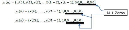
Two N-point DFTs are multiplied: Ym(k) = H(k).Xm(k), where k = 0,,1,2,….,N-1
IDFT [Ym(k)] produces blocks of length N which are not affected by aliasing as the size of DFT is N = L+M-1 and increased lengths of the sequences to N-points by appending M-1 zeros to each block.
Last M-1 points of each block must be overlapped and added to first M-1 points of the succeeding block.
(reason: Each data block terminates with M-1 zeros)
Hence, this method is known Overlap-add method. Thus, we get −
y(n) = {y1(0), y1(1), y1(2), ... .., y1(L-1), y1(L)+y2(0), y1(L+1)+y2(1), ... ... .., y1(N-1)+y2(M-1),y2(M), ... ... ... ... ... }
DSP - DFT Discrete Cosine Transform
DCT (Discrete Cosine Transform) is an N-input sequence x(n) , 0≤n≤N-1 , as a linear transformation or combination of complex exponentials. As a result, the DFT coefficients are in general, complex even if x(n) is real.
Suppose, we try to find out an orthogonal transformation which has N×N structure that expressed a real sequence x(n) as a linear combination of cosine sequence. We already know that −
$X(K) = \displaystyle\sum\limits_{n = 0}^{N-1}x(n)cos\frac{2\Pi kn}{N}0\leq k \leq N-1$
And $x(n) = \frac{1}{N}\sum_{k = 0}^{N-1}x(k)cos\frac{2\Pi kn}{N}0\leq k \leq N-1$
This is possible if N point sequence x(n) is real and even. Thus, $x(n) = x(N-n),0\leq n \leq (N-1)$. The resulting DFT itself is real and even. These things make it clear that we could possibly device a discrete cosine transform, for any N point real sequence by taking the 2N point DFT of an “Even extension” of sequence.
DCT is, basically, used in image and speech processing. It is also used in compression of images and speech signals.
$DFT[s(n)] = S(k) = \sum_{n = 0}^{2N-1}s(n)W_{2N}^{nk},\quad where\quad 0\leq k \leq 2N-1$
$S(k) = \displaystyle\sum\limits_{n = 0}^{N-1}x(n)W_{2N}^{nk}+\displaystyle\sum\limits_{n = N}^{2N-1}x(2N-n-1)W_{2N}^{nk};\quad where\quad 0\leq k\leq 2N-1$
$\Rightarrow S(k) = W_{2N}^{-k/2}+\sum_{n = 0}^{N-1}x(n) [W_{2N}^{nk}W_{2N}^{k/2}+W_{2N}^{-nk}W_{2N}^{-k/2}];\quad where\quad 0\leq k\leq 2N-1$
$\Rightarrow S(k) = W_{2N}^{\frac{k}{2}}\sum_{n = 0}^{N-1}x(n)\cos [\frac{\pi}{N}(n+\frac{1}{2})k];\quad where\quad 0\leq k\leq 2N-1$
DCT is defined by,
$V(k) = 2\sum_{n = 0}^{N-1}x(n)\cos [\frac{\pi}{2}(n+\frac{1}{2})k]\quad where\quad 0\leq k\leq N-1$
$\Rightarrow V(k) = W_{2N}^{\frac{k}{2}}S(k)\quad or\quad S(k) = W_{2N}^{\frac{k}{2}}V(k),\quad where\quad 0\leq k\leq N-1$
$\Rightarrow V(k) = 2R[W_{2N}^{\frac{k}{2}}\sum_{n = 0}^{N-1}x(n)W_{2N}^{nk}],\quad where\quad 0\leq k\leq N-1$
DSP - DFT Solved Examples
Example 1
Verify Parseval’s theorem of the sequence $x(n) = \frac{1^n}{4}u(n)$
Solution − $\displaystyle\sum\limits_{-\infty}^\infty|x_1(n)|^2 = \frac{1}{2\pi}\int_{-\pi}^{\pi}|X_1(e^{j\omega})|^2d\omega$
L.H.S $\displaystyle\sum\limits_{-\infty}^\infty|x_1(n)|^2$
$= \displaystyle\sum\limits_{-\infty}^{\infty}x(n)x^*(n)$
$= \displaystyle\sum\limits_{-\infty}^\infty(\frac{1}{4})^{2n}u(n) = \frac{1}{1-\frac{1}{16}} = \frac{16}{15}$
R.H.S. $X(e^{j\omega}) = \frac{1}{1-\frac{1}{4}e-j\omega} = \frac{1}{1-0.25\cos \omega+j0.25\sin \omega}$
$\Longleftrightarrow X^*(e^{j\omega}) = \frac{1}{1-0.25\cos \omega-j0.25\sin \omega}$
Calculating, $X(e^{j\omega}).X^*(e^{j\omega})$
$= \frac{1}{(1-0.25\cos \omega)^2+(0.25\sin \omega)^2} = \frac{1}{1.0625-0.5\cos \omega}$
$\frac{1}{2\pi}\int_{-\pi}^{\pi}\frac{1}{1.0625-0.5\cos \omega}d\omega$
$\frac{1}{2\pi}\int_{-\pi}^{\pi}\frac{1}{1.0625-0.5\cos \omega}d\omega = 16/15$
We can see that, LHS = RHS.(Hence Proved)
Example 2
Compute the N-point DFT of $x(n) = 3\delta (n)$
Solution − We know that,
$X(K) = \displaystyle\sum\limits_{n = 0}^{N-1}x(n)e^{\frac{j2\Pi kn}{N}}$
$= \displaystyle\sum\limits_{n = 0}^{N-1}3\delta(n)e^{\frac{j2\Pi kn}{N}}$
$ = 3\delta (0)\times e^0 = 1$
So,$x(k) = 3,0\leq k\leq N-1$… Ans.
Example 3
Compute the N-point DFT of $x(n) = 7(n-n_0)$
Solution − We know that,
$X(K) = \displaystyle\sum\limits_{n = 0}^{N-1}x(n)e^{\frac{j2\Pi kn}{N}}$
Substituting the value of x(n),
$\displaystyle\sum\limits_{n = 0}^{N-1}7\delta (n-n_0)e^{-\frac{j2\Pi kn}{N}}$
$= e^{-kj14\Pi kn_0/N}$… Ans
DSP - Fast Fourier Transform
In earlier DFT methods, we have seen that the computational part is too long. We want to reduce that. This can be done through FFT or fast Fourier transform. So, we can say FFT is nothing but computation of discrete Fourier transform in an algorithmic format, where the computational part will be reduced.
The main advantage of having FFT is that through it, we can design the FIR filters. Mathematically, the FFT can be written as follows;
$$x[K] = \displaystyle\sum\limits_{n = 0}^{N-1}x[n]W_N^{nk}$$Let us take an example to understand it better. We have considered eight points named from $x_0\quad to\quad x_7$. We will choose the even terms in one group and the odd terms in the other. Diagrammatic view of the above said has been shown below −
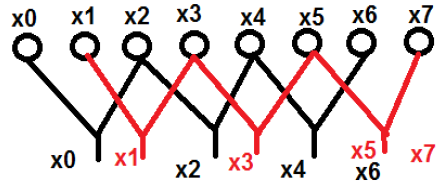
Here, points x0, x2, x4 and x6 have been grouped into one category and similarly, points x1, x3, x5 and x7 has been put into another category. Now, we can further make them in a group of two and can proceed with the computation. Now, let us see how these breaking into further two is helping in computation.
$x[k] = \displaystyle\sum\limits_{r = 0}^{\frac{N}{2}-1}x[2r]W_N^{2rk}+\displaystyle\sum\limits_{r = 0}^{\frac{N}{2}-1}x[2r+1]W_N^{(2r+1)k}$
$= \sum_{r = 0}^{\frac{N}{2}-1}x[2r]W_{N/2}^{rk}+\sum_{r = 0}^{\frac{N}{2}-1}x[2r+1]W_{N/2}^{rk}\times W_N^k$
$= G[k]+H[k]\times W_N^k$
Initially, we took an eight-point sequence, but later we broke that one into two parts G[k] and H[k]. G[k] stands for the even part whereas H[k] stands for the odd part. If we want to realize it through a diagram, then it can be shown as below −
![Eight Point H[k]G[k]1](/digital_signal_processing/images/eight_point_h_g1.jpg)
![Eight Point H[k]G[k]2](/digital_signal_processing/images/eight_point_h_g2.jpg)
From the above figure, we can see that
$W_8^4 = -1$
$W_8^5 = -W_8^1$
$W_8^6 = -W_8^2$
$W_8^7 = -W_8^3$
Similarly, the final values can be written as follows −
$G[0]-H[0] = x[4]$
$G[1]-W_8^1H[1] = x[5]$
$G[2]-W_8^2H[2] = x[6]$
$G[1]-W_8^3H[3] = x[7]$
The above one is a periodic series. The disadvantage of this system is that K cannot be broken beyond 4 point. Now Let us break down the above into further. We will get the structures something like this
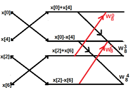
Example
Consider the sequence x[n]={ 2,1,-1,-3,0,1,2,1}. Calculate the FFT.
Solution − The given sequence is x[n]={ 2,1,-1,-3,0,1,2,1}
Arrange the terms as shown below;
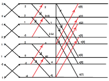
DSP - In-Place Computation
This efficient use of memory is important for designing fast hardware to calculate the FFT. The term in-place computation is used to describe this memory usage.
Decimation in Time Sequence
In this structure, we represent all the points in binary format i.e. in 0 and 1. Then, we reverse those structures. The sequence we get after that is known as bit reversal sequence. This is also known as decimation in time sequence. In-place computation of an eight-point DFT is shown in a tabular format as shown below −
| POINTS | BINARY FORMAT | REVERSAL | EQUIVALENT POINTS |
|---|---|---|---|
| 0 | 000 | 000 | 0 |
| 1 | 001 | 100 | 4 |
| 2 | 010 | 010 | 2 |
| 3 | 011 | 110 | 6 |
| 4 | 100 | 001 | 1 |
| 5 | 101 | 101 | 5 |
| 6 | 110 | 011 | 3 |
| 7 | 111 | 111 | 7 |
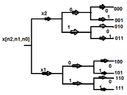
Decimation in Frequency Sequence
Apart from time sequence, an N-point sequence can also be represented in frequency. Let us take a four-point sequence to understand it better.
Let the sequence be $x[0], x[1], x[2], x[3], x[4], x[5], x[6], x[7]$. We will group two points into one group, initially. Mathematically, this sequence can be written as;
$$x[k] = \sum_{n = 0}^{N-1}x[n]W_N^{n-k}$$Now let us make one group of sequence number 0 to 3 and another group of sequence 4 to 7. Now, mathematically this can be shown as;
$$\displaystyle\sum\limits_{n = 0}^{\frac{N}{2}-1}x[n]W_N^{nk}+\displaystyle\sum\limits_{n = N/2}^{N-1}x[n]W_N^{nk}$$Let us replace n by r, where r = 0, 1 , 2….(N/2-1). Mathematically,
$$\displaystyle\sum\limits_{n = 0}^{\frac{N}{2}-1}x[r]W_{N/2}^{nr}$$We take the first four points (x[0], x[1], x[2], x[3]) initially, and try to represent them mathematically as follows −
$\sum_{n = 0}^3x[n]W_8^{nk}+\sum_{n = 0}^3x[n+4]W_8^{(n+4)k}$
$= \lbrace \sum_{n = 0}^3x[n]+\sum_{n = 0}^3x[n+4]W_8^{(4)k}\rbrace \times W_8^{nk}$
now $X[0] = \sum_{n = 0}^3(X[n]+X[n+4])$
$X[1] = \sum_{n = 0}^3(X[n]+X[n+4])W_8^{nk}$
$= [X[0]-X[4]+(X[1]-X[5])W_8^1+(X[2]-X[6])W_8^2+(X[3]-X[7])W_8^3$
We can further break it into two more parts, which means instead of breaking them as 4-point sequence, we can break them into 2-point sequence.
DSP - Computer Aided Design
FIR filters can be useful in making computer-aided design of the filters. Let us take an example and see how it works. Given below is a figure of desired filter.
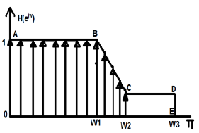
While doing computer designing, we break the whole continuous graph figures into discrete values. Within certain limits, we break it into either 64, 256 or 512 (and so on) number of parts having discrete magnitudes.
In the above example, we have taken limits between -π to +π. We have divided it into 256 parts. The points can be represented as H(0), H(1),….up to H(256). Here, we apply IDFT algorithm and this will give us linear phase characteristics.
Sometimes, we may be interested in some particular order of filter. Let us say we want to realize the above given design through 9th order filter. So, we take filter values as h0, h1, h2….h9. Mathematically, it can be shown as below
$$H(e^{j\omega}) = h_0+h_1e^{-j\omega}+h_2e^{-2j\omega}+.....+h_9e^{-9j\omega}$$Where there are large number of dislocations, we take maximum points.
For example, in the above figure, there is a sudden drop of slopping between the points B and C. So, we try to take more discrete values at this point, but there is a constant slope between point C and D. There we take less number of discrete values.
For designing the above filter, we go through minimization process as follows;
$H(e^{j\omega1}) = h_0+h_1e^{-j\omega1}+h_2e^{-2j\omega1}+.....+h_9e^{-9j\omega1}$
$H(e^{j\omega2}) = h_0+h_1e^{-j\omega2}+h_2e^{-2j\omega2}+.....+h_9e^{-9j\omega2}$
Similarly,
$(e^{j\omega1000}) = h_0+h_1eH^{-j\omega1000}h_2e^{-2j\omega1000}+.....+h_9+e^{-9j\omega1000}$
Representing the above equation in matrix form, we have −
$$\begin{bmatrix}H(e^{j\omega_1})\\.\\.\\H(e^{j\omega_{1000}}) \end{bmatrix} = \begin{bmatrix}e^{-j\omega_1} & ... & e^{-j9\omega_1} \\. & & . \\. & & . \\e^{-j\omega_{1000}} &... & e^{j9\omega_{1000}} \end{bmatrix}\begin{bmatrix}h_0\\.\\.\\h_9\end{bmatrix}$$Let us take the 1000×1 matrix as B, 1000×9 matrix as A and 9×1 matrix as $\hat{h}$.
So, for solving the above matrix, we will write
$\hat{h} = [A^TA]^{-1}A^{T}B$
$= [A^{*T}A]^{-1}A^{*T}B$
where A* represents the complex conjugate of the matrix A.