- Data Structures & Algorithms
- DSA - Home
- DSA - Overview
- DSA - Environment Setup
- DSA - Algorithms Basics
- DSA - Asymptotic Analysis
- Data Structures
- DSA - Data Structure Basics
- DSA - Data Structures and Types
- DSA - Array Data Structure
- Linked Lists
- DSA - Linked List Data Structure
- DSA - Doubly Linked List Data Structure
- DSA - Circular Linked List Data Structure
- Stack & Queue
- DSA - Stack Data Structure
- DSA - Expression Parsing
- DSA - Queue Data Structure
- Searching Algorithms
- DSA - Searching Algorithms
- DSA - Linear Search Algorithm
- DSA - Binary Search Algorithm
- DSA - Interpolation Search
- DSA - Jump Search Algorithm
- DSA - Exponential Search
- DSA - Fibonacci Search
- DSA - Sublist Search
- DSA - Hash Table
- Sorting Algorithms
- DSA - Sorting Algorithms
- DSA - Bubble Sort Algorithm
- DSA - Insertion Sort Algorithm
- DSA - Selection Sort Algorithm
- DSA - Merge Sort Algorithm
- DSA - Shell Sort Algorithm
- DSA - Heap Sort
- DSA - Bucket Sort Algorithm
- DSA - Counting Sort Algorithm
- DSA - Radix Sort Algorithm
- DSA - Quick Sort Algorithm
- Graph Data Structure
- DSA - Graph Data Structure
- DSA - Depth First Traversal
- DSA - Breadth First Traversal
- DSA - Spanning Tree
- Tree Data Structure
- DSA - Tree Data Structure
- DSA - Tree Traversal
- DSA - Binary Search Tree
- DSA - AVL Tree
- DSA - Red Black Trees
- DSA - B Trees
- DSA - B+ Trees
- DSA - Splay Trees
- DSA - Tries
- DSA - Heap Data Structure
- Recursion
- DSA - Recursion Algorithms
- DSA - Tower of Hanoi Using Recursion
- DSA - Fibonacci Series Using Recursion
- Divide and Conquer
- DSA - Divide and Conquer
- DSA - Max-Min Problem
- DSA - Strassen's Matrix Multiplication
- DSA - Karatsuba Algorithm
- Greedy Algorithms
- DSA - Greedy Algorithms
- DSA - Travelling Salesman Problem (Greedy Approach)
- DSA - Prim's Minimal Spanning Tree
- DSA - Kruskal's Minimal Spanning Tree
- DSA - Dijkstra's Shortest Path Algorithm
- DSA - Map Colouring Algorithm
- DSA - Fractional Knapsack Problem
- DSA - Job Sequencing with Deadline
- DSA - Optimal Merge Pattern Algorithm
- Dynamic Programming
- DSA - Dynamic Programming
- DSA - Matrix Chain Multiplication
- DSA - Floyd Warshall Algorithm
- DSA - 0-1 Knapsack Problem
- DSA - Longest Common Subsequence Algorithm
- DSA - Travelling Salesman Problem (Dynamic Approach)
- Approximation Algorithms
- DSA - Approximation Algorithms
- DSA - Vertex Cover Algorithm
- DSA - Set Cover Problem
- DSA - Travelling Salesman Problem (Approximation Approach)
- Randomized Algorithms
- DSA - Randomized Algorithms
- DSA - Randomized Quick Sort Algorithm
- DSA - Karger’s Minimum Cut Algorithm
- DSA - Fisher-Yates Shuffle Algorithm
- DSA Useful Resources
- DSA - Questions and Answers
- DSA - Quick Guide
- DSA - Useful Resources
- DSA - Discussion
Data Structures - Searching Algorithms

In the previous section, we have discussed various Sorting Techniques and cases in which they can be used. However, the main idea behind performing sorting is to arrange the data in an orderly way, making it easier to search for any element within the sorted data.
Searching is a process of finding a particular record, which can be a single element or a small chunk, within a huge amount of data. The data can be in various forms: arrays, linked lists, trees, heaps, and graphs etc. With the increasing amount of data nowadays, there are multiple techniques to perform the searching operation.
Searching Algorithms in Data Structures
Various searching techniques can be applied on the data structures to retrieve certain data. A search operation is said to be successful only if it returns the desired element or data; otherwise, the searching method is unsuccessful.
There are two categories these searching techniques fall into. They are −
Sequential Searching
Interval Searching
Sequential Searching
As the name suggests, the sequential searching operation traverses through each element of the data sequentially to look for the desired data. The data need not be in a sorted manner for this type of search.
Example − Linear Search
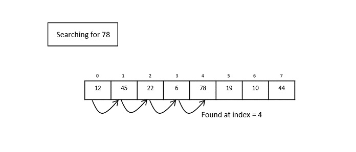
Fig. 1: Linear Search Operation
Interval Searching
Unlike sequential searching, the interval searching operation requires the data to be in a sorted manner. This method usually searches the data in intervals; it could be done by either dividing the data into multiple sub-parts or jumping through the indices to search for an element.
Example − Binary Search, Jump Search etc.
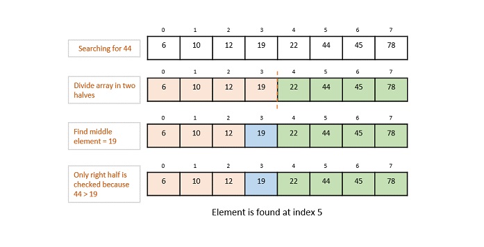
Fig. 2: Binary Search Operation
Evaluating Searching Algorithms
Usually, not all searching techniques are suitable for all types of data structures. In some cases, a sequential search is preferable while in other cases interval searching is preferable. Evaluation of these searching techniques is done by checking the running time taken by each searching method on a particular input.
This is where asymptotic notations come into the picture. To learn more about Asymptotic Notations, please click here.
To explain briefly, there are three different cases of time complexity in which a program can run. They are −
Best Case
Average Case
Worst Case
We mostly concentrate on the only best-case and worst-case time complexities, as the average case is difficult to compute. And since the running time is based on the amount of input given to the program, the worst-case time complexity best describes the performance of any algorithm.
For instance, the best case time complexity of a linear search is O(1) where the desired element is found in the first iteration; whereas the worst case time complexity is O(n) when the program traverses through all the elements and still does not find an element. This is labelled as an unsuccessful search. Therefore, the actual time complexity of a linear search is seen as O(n), where n is the number of elements present in the input data structure.
Many types of searching methods are used to search for data entries in various data structures. Some of them include −
Ubiquitous Binary Search
We will look at each of these searching methods elaborately in the following chapters.