Optimal Cost Binary Search Trees

---

---

A Binary Search Tree (BST) is a tree where the key values are stored in the internal nodes. The external nodes are null nodes. The keys are ordered lexicographically, i.e. for each internal node all the keys in the left sub-tree are less than the keys in the node, and all the keys in the right sub-tree are greater.

When we know the frequency of searching each one of the keys, it is quite easy to compute the expected cost of accessing each node in the tree. An optimal binary search tree is a BST, which has minimal expected cost of locating each node

Search time of an element in a BST is O(n), whereas in a Balanced-BST search time is O(log n). Again the search time can be improved in Optimal Cost Binary Search Tree, placing the most frequently used data in the root and closer to the root element, while placing the least frequently used data near leaves and in leaves.

Here, the Optimal Binary Search Tree Algorithm is presented. First, we build a BST from a set of provided n number of distinct keys < k₁, k₂, k₃, ... k_n >. Here we assume, the probability of accessing a key K_i is p_i. Some dummy keys (d₀, d₁, d₂, ... d_n) are added as some searches may be performed for the values which are not present in the Key set K. We assume, for each dummy key d_i probability of access is q_i.

Optimal-Binary-Search-Tree(p, q, n) 
e[1…n + 1, 0…n],  
w[1…n + 1, 0…n], 
root[1…n + 1, 0…n]  
for i = 1 to n + 1 do 
   e[i, i - 1] := qi - 1 
   w[i, i - 1] := qi - 1  
for l = 1 to n do 
   for i = 1 to n – l + 1 do 
      j = i + l – 1 e[i, j] := ∞ 
      w[i, i] := w[i, i -1] + pj + qj 
      for r = i to j do 
         t := e[i, r - 1] + e[r + 1, j] + w[i, j] 
         if t < e[i, j] 
            e[i, j] := t 
            root[i, j] := r 
return e and root 

Analysis

The algorithm requires O (n³) time, since three nested for loops are used. Each of these loops takes on at most n values.

Example

Considering the following tree, the cost is 2.80, though this is not an optimal result.

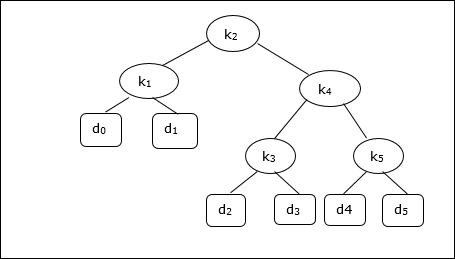
Node	Depth	Probability	Contribution
k1	1	0.15	0.30
k2	0	0.10	0.10
k3	2	0.05	0.15
k4	1	0.10	0.20
k5	2	0.20	0.60
d0	2	0.05	0.15
d1	2	0.10	0.30
d2	3	0.05	0.20
d3	3	0.05	0.20
d4	3	0.05	0.20
d5	3	0.10	0.40
Total			2.80

To get an optimal solution, using the algorithm discussed in this chapter, the following tables are generated.

In the following tables, column index is i and row index is j.

e	1	2	3	4	5	6
5	2.75	2.00	1.30	0.90	0.50	0.10
4	1.75	1.20	0.60	0.30	0.05
3	1.25	0.70	0.25	0.05
2	0.90	0.40	0.05
1	0.45	0.10
0	0.05

w	1	2	3	4	5	6
5	1.00	0.80	0.60	0.50	0.35	0.10
4	0.70	0.50	0.30	0.20	0.05
3	0.55	0.35	0.15	0.05
2	0.45	0.25	0.05
1	0.30	0.10
0	0.05

root	1	2	3	4	5
5	2	4	5	5	5
4	2	2	4	4
3	2	2	3
2	1	2
1	1

From these tables, the optimal tree can be formed.