
- Control Systems Tutorial
- Control Systems - Home
- Control Systems - Introduction
- Control Systems - Feedback
- Mathematical Models
- Modelling of Mechanical Systems
- Electrical Analogies of Mechanical Systems
- Control Systems - Block Diagrams
- Block Diagram Algebra
- Block Diagram Reduction
- Signal Flow Graphs
- Mason's Gain Formula
- Time Response Analysis
- Response of the First Order System
- Response of Second Order System
- Time Domain Specifications
- Steady State Errors
- Control Systems - Stability
- Control Systems - Stability Analysis
- Control Systems - Root Locus
- Construction of Root Locus
- Frequency Response Analysis
- Control Systems - Bode Plots
- Construction of Bode Plots
- Control Systems - Polar Plots
- Control Systems - Nyquist Plots
- Control Systems - Compensators
- Control Systems - Controllers
- Control Systems - State Space Model
- State Space Analysis
- Control Systems Useful Resources
- Control Systems - Quick Guide
- Control Systems - Useful Resources
- Control Systems - Discussion
Control Systems - Polar Plots
In the previous chapters, we discussed the Bode plots. There, we have two separate plots for both magnitude and phase as the function of frequency. Let us now discuss about polar plots. Polar plot is a plot which can be drawn between magnitude and phase. Here, the magnitudes are represented by normal values only.
The polar form of $G(j\omega)H(j\omega)$ is
$$G(j\omega)H(j\omega)=|G(j\omega)H(j\omega)| \angle G(j\omega)H(j\omega)$$
The Polar plot is a plot, which can be drawn between the magnitude and the phase angle of $G(j\omega)H(j\omega)$ by varying $\omega$ from zero to ∞. The polar graph sheet is shown in the following figure.
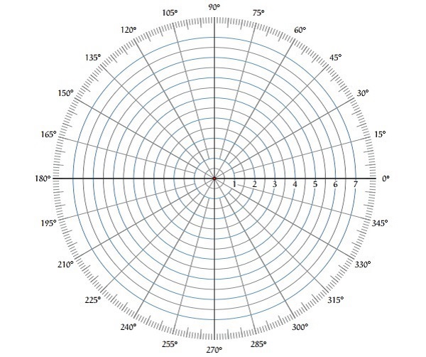
This graph sheet consists of concentric circles and radial lines. The concentric circles and the radial lines represent the magnitudes and phase angles respectively. These angles are represented by positive values in anti-clock wise direction. Similarly, we can represent angles with negative values in clockwise direction. For example, the angle 2700 in anti-clock wise direction is equal to the angle −900 in clockwise direction.
Rules for Drawing Polar Plots
Follow these rules for plotting the polar plots.
Substitute, $s = j\omega$ in the open loop transfer function.
Write the expressions for magnitude and the phase of $G(j\omega)H(j\omega)$.
Find the starting magnitude and the phase of $G(j\omega)H(j\omega)$ by substituting $\omega = 0$. So, the polar plot starts with this magnitude and the phase angle.
Find the ending magnitude and the phase of $G(j\omega)H(j\omega)$ by substituting $\omega = \infty$. So, the polar plot ends with this magnitude and the phase angle.
Check whether the polar plot intersects the real axis, by making the imaginary term of $G(j\omega)H(j\omega)$ equal to zero and find the value(s) of $\omega$.
Check whether the polar plot intersects the imaginary axis, by making real term of $G(j\omega)H(j\omega)$ equal to zero and find the value(s) of $\omega$.
For drawing polar plot more clearly, find the magnitude and phase of $G(j\omega)H(j\omega)$ by considering the other value(s) of $\omega$.
Example
Consider the open loop transfer function of a closed loop control system.
$$G(s)H(s)=\frac{5}{s(s+1)(s+2)}$$
Let us draw the polar plot for this control system using the above rules.
Step 1 − Substitute, $s = j\omega$ in the open loop transfer function.
$$G(j\omega)H(j\omega)=\frac{5}{j\omega(j\omega+1)(j\omega+2)}$$
The magnitude of the open loop transfer function is
$$M=\frac{5}{\omega(\sqrt{\omega^2+1})(\sqrt{\omega^2+4})}$$
The phase angle of the open loop transfer function is
$$\phi=-90^0-\tan^{-1}\omega-\tan^{-1}\frac{\omega}{2}$$
Step 2 − The following table shows the magnitude and the phase angle of the open loop transfer function at $\omega = 0$ rad/sec and $\omega = \infty$ rad/sec.
| Frequency (rad/sec) | Magnitude | Phase angle(degrees) |
|---|---|---|
| 0 | ∞ | -90 or 270 |
| ∞ | 0 | -270 or 90 |
So, the polar plot starts at (∞,−900) and ends at (0,−2700). The first and the second terms within the brackets indicate the magnitude and phase angle respectively.
Step 3 − Based on the starting and the ending polar co-ordinates, this polar plot will intersect the negative real axis. The phase angle corresponding to the negative real axis is −1800 or 1800. So, by equating the phase angle of the open loop transfer function to either −1800 or 1800, we will get the $\omega$ value as $\sqrt{2}$.
By substituting $\omega = \sqrt{2}$ in the magnitude of the open loop transfer function, we will get $M = 0.83$. Therefore, the polar plot intersects the negative real axis when $\omega = \sqrt{2}$ and the polar coordinate is (0.83,−1800).
So, we can draw the polar plot with the above information on the polar graph sheet.