Visible Surface Detection

When we view a picture containing non-transparent objects and surfaces, then we cannot see those objects from view which are behind from objects closer to eye. We must remove these hidden surfaces to get a realistic screen image. The identification and removal of these surfaces is called Hidden-surface problem.

There are two approaches for removing hidden surface problems − Object-Space method and Image-space method. The Object-space method is implemented in physical coordinate system and image-space method is implemented in screen coordinate system.

When we want to display a 3D object on a 2D screen, we need to identify those parts of a screen that are visible from a chosen viewing position.

Depth Buffer (Z-Buffer) Method

This method is developed by Cutmull. It is an image-space approach. The basic idea is to test the Z-depth of each surface to determine the closest (visible) surface.

In this method each surface is processed separately one pixel position at a time across the surface. The depth values for a pixel are compared and the closest (smallest z) surface determines the color to be displayed in the frame buffer.

It is applied very efficiently on surfaces of polygon. Surfaces can be processed in any order. To override the closer polygons from the far ones, two buffers named frame buffer and depth buffer, are used.

Depth buffer is used to store depth values for (x, y) position, as surfaces are processed (0 ≤ depth ≤ 1).

The frame buffer is used to store the intensity value of color value at each position (x, y).

The z-coordinates are usually normalized to the range [0, 1]. The 0 value for z-coordinate indicates back clipping pane and 1 value for z-coordinates indicates front clipping pane.

Algorithm

Step-1 − Set the buffer values −

Depthbuffer (x, y) = 0

Framebuffer (x, y) = background color

Step-2 − Process each polygon (One at a time)

For each projected (x, y) pixel position of a polygon, calculate depth z.

If Z > depthbuffer (x, y)

Compute surface color,

set depthbuffer (x, y) = z,

framebuffer (x, y) = surfacecolor (x, y)

Advantages

It is easy to implement.
It reduces the speed problem if implemented in hardware.
It processes one object at a time.

Disadvantages

It requires large memory.
It is time consuming process.

Scan-Line Method

It is an image-space method to identify visible surface. This method has a depth information for only single scan-line. In order to require one scan-line of depth values, we must group and process all polygons intersecting a given scan-line at the same time before processing the next scan-line. Two important tables, edge table and polygon table, are maintained for this.

The Edge Table − It contains coordinate endpoints of each line in the scene, the inverse slope of each line, and pointers into the polygon table to connect edges to surfaces.

The Polygon Table − It contains the plane coefficients, surface material properties, other surface data, and may be pointers to the edge table.

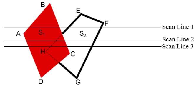
To facilitate the search for surfaces crossing a given scan-line, an active list of edges is formed. The active list stores only those edges that cross the scan-line in order of increasing x. Also a flag is set for each surface to indicate whether a position along a scan-line is either inside or outside the surface.

Pixel positions across each scan-line are processed from left to right. At the left intersection with a surface, the surface flag is turned on and at the right, the flag is turned off. You only need to perform depth calculations when multiple surfaces have their flags turned on at a certain scan-line position.

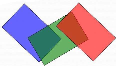
Area-Subdivision Method

The area-subdivision method takes advantage by locating those view areas that represent part of a single surface. Divide the total viewing area into smaller and smaller rectangles until each small area is the projection of part of a single visible surface or no surface at all.

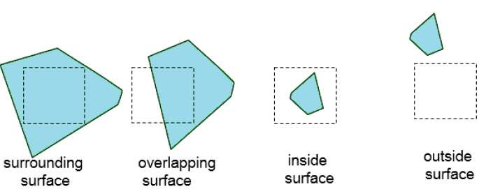
Continue this process until the subdivisions are easily analyzed as belonging to a single surface or until they are reduced to the size of a single pixel. An easy way to do this is to successively divide the area into four equal parts at each step. There are four possible relationships that a surface can have with a specified area boundary.

Surrounding surface − One that completely encloses the area.
Overlapping surface − One that is partly inside and partly outside the area.
Inside surface − One that is completely inside the area.
Outside surface − One that is completely outside the area.

The tests for determining surface visibility within an area can be stated in terms of these four classifications. No further subdivisions of a specified area are needed if one of the following conditions is true −

All surfaces are outside surfaces with respect to the area.
Only one inside, overlapping or surrounding surface is in the area.
A surrounding surface obscures all other surfaces within the area boundaries.

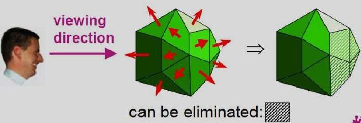
Back-Face Detection

A fast and simple object-space method for identifying the back faces of a polyhedron is based on the "inside-outside" tests. A point (x, y, z) is "inside" a polygon surface with plane parameters A, B, C, and D if When an inside point is along the line of sight to the surface, the polygon must be a back face (we are inside that face and cannot see the front of it from our viewing position).

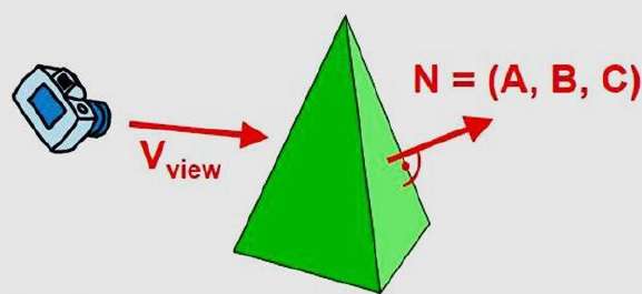
We can simplify this test by considering the normal vector N to a polygon surface, which has Cartesian components (A, B, C).

In general, if V is a vector in the viewing direction from the eye (or "camera") position, then this polygon is a back face if

V.N > 0

Furthermore, if object descriptions are converted to projection coordinates and your viewing direction is parallel to the viewing z-axis, then −

V = (0, 0, V_z) and V.N = V_ZC

So that we only need to consider the sign of C the component of the normal vector N.

In a right-handed viewing system with viewing direction along the negative $Z_{V}$ axis, the polygon is a back face if C < 0. Also, we cannot see any face whose normal has z component C = 0, since your viewing direction is towards that polygon. Thus, in general, we can label any polygon as a back face if its normal vector has a z component value −

C <= 0

Similar methods can be used in packages that employ a left-handed viewing system. In these packages, plane parameters A, B, C and D can be calculated from polygon vertex coordinates specified in a clockwise direction (unlike the counterclockwise direction used in a right-handed system).

Also, back faces have normal vectors that point away from the viewing position and are identified by C >= 0 when the viewing direction is along the positive $Z_{v}$ axis. By examining parameter C for the different planes defining an object, we can immediately identify all the back faces.

A-Buffer Method

The A-buffer method is an extension of the depth-buffer method. The A-buffer method is a visibility detection method developed at Lucas film Studios for the rendering system Renders Everything You Ever Saw (REYES).

The A-buffer expands on the depth buffer method to allow transparencies. The key data structure in the A-buffer is the accumulation buffer.

Each position in the A-buffer has two fields −

Depth field − It stores a positive or negative real number
Intensity field − It stores surface-intensity information or a pointer value

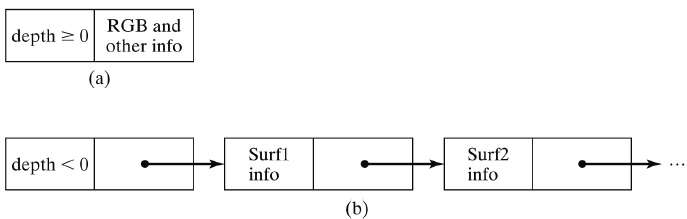
If depth >= 0, the number stored at that position is the depth of a single surface overlapping the corresponding pixel area. The intensity field then stores the RGB components of the surface color at that point and the percent of pixel coverage.

If depth < 0, it indicates multiple-surface contributions to the pixel intensity. The intensity field then stores a pointer to a linked list of surface data. The surface buffer in the A-buffer includes −

RGB intensity components
Opacity Parameter
Depth
Percent of area coverage
Surface identifier

The algorithm proceeds just like the depth buffer algorithm. The depth and opacity values are used to determine the final color of a pixel.

Depth Sorting Method

Depth sorting method uses both image space and object-space operations. The depth-sorting method performs two basic functions −

First, the surfaces are sorted in order of decreasing depth.
Second, the surfaces are scan-converted in order, starting with the surface of greatest depth.

The scan conversion of the polygon surfaces is performed in image space. This method for solving the hidden-surface problem is often referred to as the painter's algorithm. The following figure shows the effect of depth sorting −

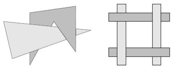
The algorithm begins by sorting by depth. For example, the initial “depth” estimate of a polygon may be taken to be the closest z value of any vertex of the polygon.

Let us take the polygon P at the end of the list. Consider all polygons Q whose z-extents overlap P’s. Before drawing P, we make the following tests. If any of the following tests is positive, then we can assume P can be drawn before Q.

Do the x-extents not overlap?
Do the y-extents not overlap?
Is P entirely on the opposite side of Q’s plane from the viewpoint?
Is Q entirely on the same side of P’s plane as the viewpoint?
Do the projections of the polygons not overlap?

If all the tests fail, then we split either P or Q using the plane of the other. The new cut polygons are inserting into the depth order and the process continues. Theoretically, this partitioning could generate O(n²) individual polygons, but in practice, the number of polygons is much smaller.

Binary Space Partition (BSP) Trees

Binary space partitioning is used to calculate visibility. To build the BSP trees, one should start with polygons and label all the edges. Dealing with only one edge at a time, extend each edge so that it splits the plane in two. Place the first edge in the tree as root. Add subsequent edges based on whether they are inside or outside. Edges that span the extension of an edge that is already in the tree are split into two and both are added to the tree.

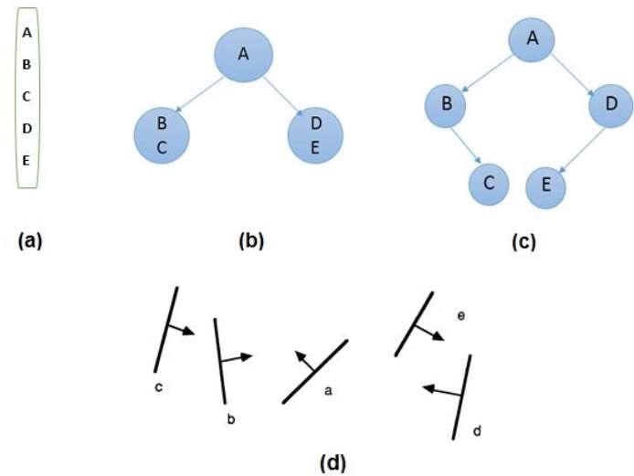
From the above figure, first take A as a root.
Make a list of all nodes in figure (a).
Put all the nodes that are in front of root A to the left side of node A and put all those nodes that are behind the root A to the right side as shown in figure (b).
Process all the front nodes first and then the nodes at the back.
As shown in figure (c), we will first process the node B. As there is nothing in front of the node B, we have put NIL. However, we have node C at back of node B, so node C will go to the right side of node B.
Repeat the same process for the node D.