- Big Data Analytics Tutorial
- Big Data Analytics - Home
- Big Data Analytics - Overview
- Big Data Analytics - Data Life Cycle
- Big Data Analytics - Methodology
- Core Deliverables
- Key Stakeholders
- Big Data Analytics - Data Analyst
- Big Data Analytics - Data Scientist
- Big Data Analytics Project
- Data Analytics - Problem Definition
- Big Data Analytics - Data Collection
- Big Data Analytics - Cleansing data
- Big Data Analytics - Summarizing
- Big Data Analytics - Data Exploration
- Data Visualization
- Big Data Analytics Methods
- Big Data Analytics - Introduction to R
- Data Analytics - Introduction to SQL
- Big Data Analytics - Charts & Graphs
- Big Data Analytics - Data Tools
- Data Analytics - Statistical Methods
- Advanced Methods
- Machine Learning for Data Analysis
- Naive Bayes Classifier
- K-Means Clustering
- Association Rules
- Big Data Analytics - Decision Trees
- Logistic Regression
- Big Data Analytics - Time Series
- Big Data Analytics - Text Analytics
- Big Data Analytics - Online Learning
- Big Data Analytics Useful Resources
- Big Data Analytics - Quick Guide
- Big Data Analytics - Resources
- Big Data Analytics - Discussion
Big Data Analytics - Data Exploration
Exploratory data analysis is a concept developed by John Tuckey (1977) that consists on a new perspective of statistics. Tuckey’s idea was that in traditional statistics, the data was not being explored graphically, is was just being used to test hypotheses. The first attempt to develop a tool was done in Stanford, the project was called prim9. The tool was able to visualize data in nine dimensions, therefore it was able to provide a multivariate perspective of the data.
In recent days, exploratory data analysis is a must and has been included in the big data analytics life cycle. The ability to find insight and be able to communicate it effectively in an organization is fueled with strong EDA capabilities.
Based on Tuckey’s ideas, Bell Labs developed the S programming language in order to provide an interactive interface for doing statistics. The idea of S was to provide extensive graphical capabilities with an easy-to-use language. In today’s world, in the context of Big Data, R that is based on the S programming language is the most popular software for analytics.
The following program demonstrates the use of exploratory data analysis.
The following is an example of exploratory data analysis. This code is also available in part1/eda/exploratory_data_analysis.R file.
library(nycflights13)
library(ggplot2)
library(data.table)
library(reshape2)
# Using the code from the previous section
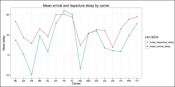
# This computes the mean arrival and departure delays by carrier.
DT <- as.data.table(flights)
mean2 = DT[, list(mean_departure_delay = mean(dep_delay, na.rm = TRUE),
mean_arrival_delay = mean(arr_delay, na.rm = TRUE)),
by = carrier]
# In order to plot data in R usign ggplot, it is normally needed to reshape the data
# We want to have the data in long format for plotting with ggplot
dt = melt(mean2, id.vars = ’carrier’)
# Take a look at the first rows
print(head(dt))
# Take a look at the help for ?geom_point and geom_line to find similar examples
# Here we take the carrier code as the x axis
# the value from the dt data.table goes in the y axis
# The variable column represents the color
p = ggplot(dt, aes(x = carrier, y = value, color = variable, group = variable)) +
geom_point() + # Plots points
geom_line() + # Plots lines
theme_bw() + # Uses a white background
labs(list(title = 'Mean arrival and departure delay by carrier',
x = 'Carrier', y = 'Mean delay'))
print(p)
# Save the plot to disk
ggsave('mean_delay_by_carrier.png', p,
width = 10.4, height = 5.07)
The code should produce an image such as the following −